Distance based plots

Forest Inventory lecturenotes

Category Forest Inventory lecturenotes not found

Figure 1 Some variations of k-tree sampling (Kleinn 2007).

Figure 2 Illustration why the simple expansion factor approach does produce a systematic overestimation for k-tree sampling (Kleinn 2007).

Point-to-tree distance techniques are also applied in ecological studies in which the k nearest objects (trees or plants) to a sample point are selected and constitute the set of sample objects for that particular sample plot. The idea of point-to-tree distance sampling is striking, because it greatly facilitates field work (if the values of k are not too big) under many conditions. All sample plots contain the same number of k trees, so that both empty plots and very high frequency plots are avoided. Because of the fixed number of trees (objects), this class of response designs is also referred to as fixed-count distance methods while in the context of ecological methodology it is also referred to as plotless methods because there is no need to lay out a fixed plot area.

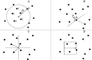
Here we use the term k-tree sampling to indicate that it is a generalized fixed number of objects that are to be counted. While applications of k-tree sampling can be found in many fields (Engeman et al. 1994, for example, mention density estimation of colonial-nesting seabirds and density of rat damage in sugar cane), we focus here on the forestry context where - in addition to density - many more tree attributes are to be estimated. Some variations of k-tree distance sampling are depicted in Figure 63. The 6-tree technique was proposed by Prodan (1968) and is still being used for forest management inventories in South Western Germany. Prodan (1968) and Schöpfer (1969a,b) found that a k-value of 6 had optimal properties in terms of practical applicability and statistical performance.

T‑square sampling and the point centered quarter (PCQ) method (Figure 63 B and C) are mainly used in ecological sampling studies and in particular for density estimation; they may be seen as “restricted point-to-tree distance techniques” because they introduce further conditions for the selection of the sample trees, mainly in order to reduce the possibility that among the k selected trees there are pairs of trees very close together: in the T square technique (k=2), the tree closest to the sample point is selected; but then the second tree to be selected is the one closest to the first closest tree on the side opposite to the sample point. It therefore is a combination of point-to-tree and tree-to-tree distance sampling. While T-square sampling is usually presented for k=2, one could extend it to the selection of more trees along the rule defined for the selection of the second tree.

In the PCQ method, four quadrants are established around the sample point and in each quadrant the tree closest to the sample point is selected so that k=4. Variations of this technique include subdividing the space around the sample points into numbers other than j=4 equal sections. Another variation would be to select m>1 trees in each of the j sectors, forming a k=mj sample. k-tree sampling may also be implemented as a transect of fixed width and variable length (see Figure 63 C) where the transect is being extended until the k-tree is reached.

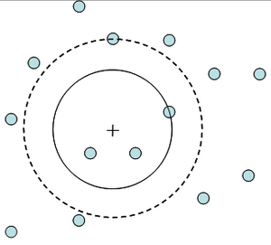
We focus here on case A in Figure 63, the unrestricted k-tree distance sampling. A common approach to estimation from fixed area plots is to calculate an expansion factor which converts the per-plot values to their equivalent per hectare; to calculate the expansion factor a plot area needs to be defined which obviously depends in some way on the distances between the sample point and the k trees. By using a seemingly straightforward approach and defining the plot area as a circle with radius equal to the distance to the k tree, however, we produce a systematic overestimation, i.e. a positive estimator bias. Taking the area defined by the distance to the k tree we are establishing the smallest possible circular plot and this in turn yields the largest possible expansion factor. If we extended the radius up to but not including the k+1 tree, there would still be k trees within the plot but the expansion factor would be smaller! This is illustrated in Figure 64. If we follow the expansion factor approach, it is obvious that the correct plot radius must be somewhere between the distance to the k tree and the distance to the k-1 tree. In a simulation study, Kleinn and Vilcko (2006a) showed that the circle plot through the k tree produces a systematic overestimation and the circle plot through the k+1 tree produces a systematic underestimation; where, of course, for increasing values of k the bias becomes smaller and smaller. This is illustrated in Figure 65.

References

- ↑ 1.0 1.1 Kleinn, C. 2007. Lecture Notes for the Teaching Module Forest Inventory. Department of Forest Inventory and Remote Sensing. Faculty of Forest Science and Forest Ecology, Georg-August-Universität Göttingen. 164 S.