Creating jigsaw puzzles in ArcMap

The concept of cluster inclusionzones for fixed area sample plots

The so called jigsaw puzzle view (Roesch et al. 1993) is a decomopsition of the total domain of interest in non-overlapping inclusion zones for exclusive clusters of trees. In the infinite population approach sample elements are dimensionless points drawn from an infinite sample frame. On the other side we can only imagine a certain discrete number of possible realizations of a target variable as observations are derived as generalization over a number of nearest neighbours (trees) to a certain sample point. In fixed area sampling neighbours are considered up to a fixed distance (the radius of a circular sample plot). This "inclusion distance" can be assigned to every tree in the domain of interest, as a sample point falling in that distance would lead to a selection of the respective tree. This single tree inclusion zones are overlapping (as in most cases more than only one tree is selected by a sample point) whereas the resulting pattern is a decomposition of the total area in non-overlapping polygons, that would lead to a selection of a particular cluster of trees. As the number of possible observations (derived from clusters) is much smaller than the invinite number of possible sample points, the jigsaw puzzle is a classification of the infinite sample frame in areas of possible realizations. The size of the polygons is an expression of the selection probability for a certain observation. This article describes briefly, how jigsaw puzzles can be created from a map with tree locations in ArcGIS.

Workflow of creating jigsaw puzzles

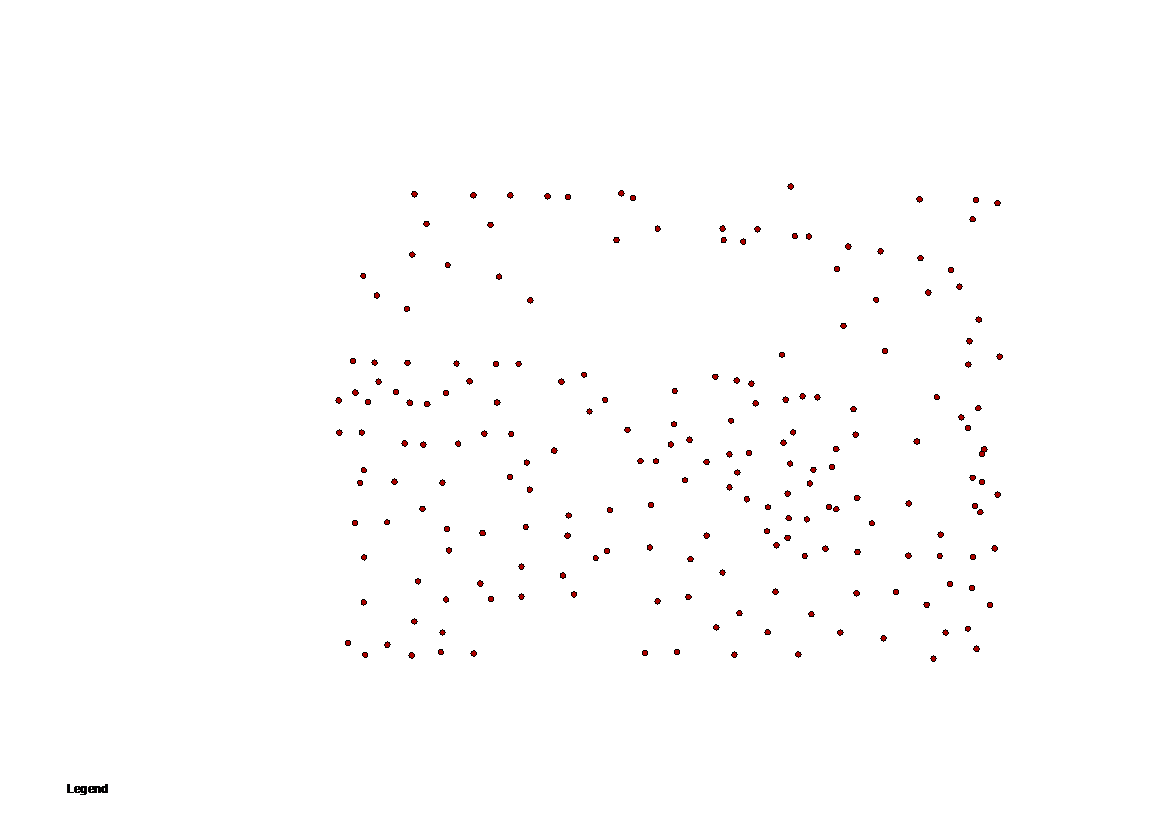
• Basis for this decomposition is a map with tree locations (x and y coordinates) that might be generated or the result of a full assessment of a forest stand as shapefile or layer.

Creating buffers

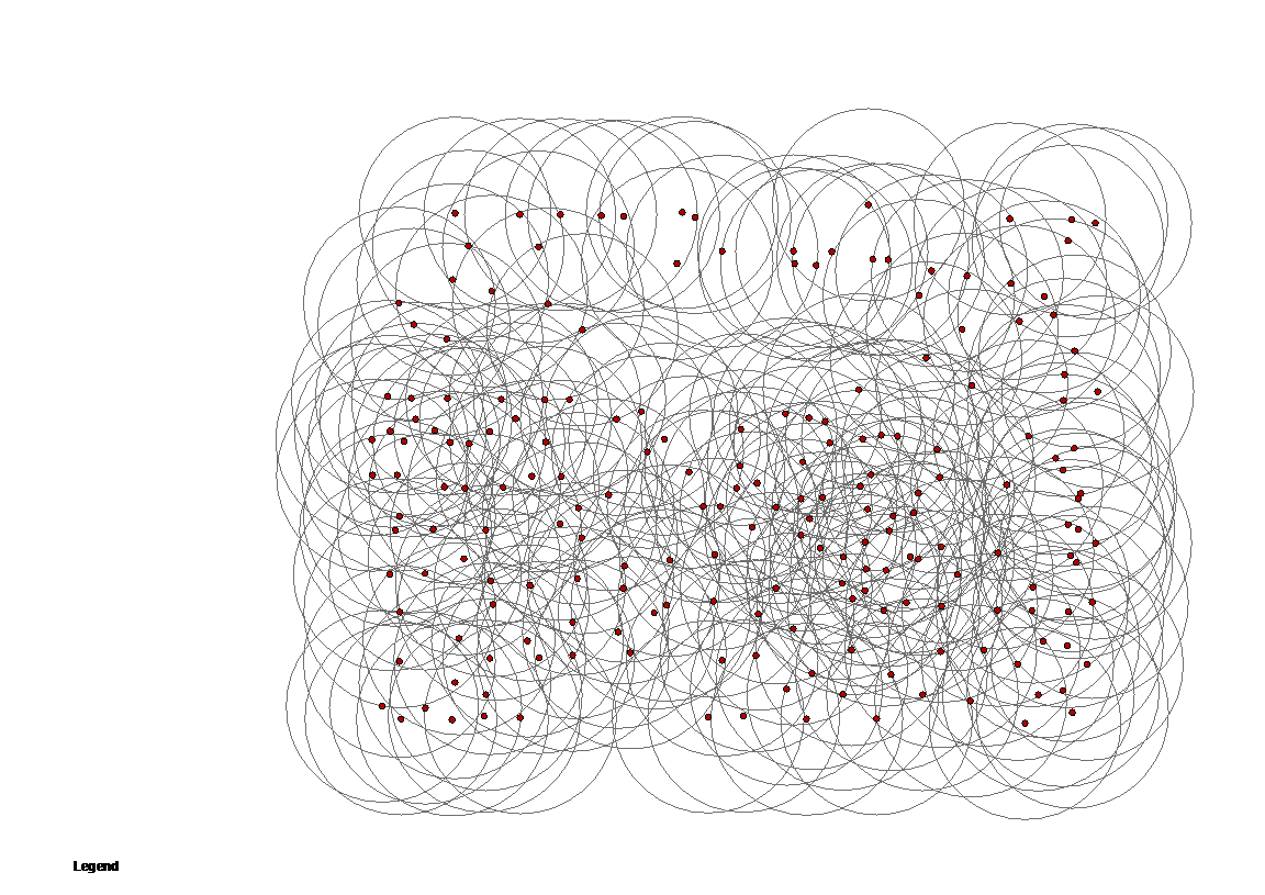
• All trees must be buffered with the radius of a cirlular sample plot (their inclusion zone). Therefor create a new empty shapefile for polygons (with ArcCatalog) and load it to ArcMap. Start editing the tree-shape and select the new empty polygon shapefile as target for creating new features. Choose Buffer from the edit menu.

• After buffering all points your output looks like this:

"Union"

• The next step is to identify all overlapping polygons and the resulting number of selected inclusion zones for the particular area. Therefore one has to add a new column to the data table (of the buffer shape) for the number of stems that are related to the specific inclusion zones. As every inclusion zone is exclusive for only one tree, this column contains the value 1 for all buffer polygons (use the field calculator and set the new field =1 for all).

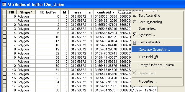
• Now we create a new layer containing all resulting polygons by Union all buffers. Therefore select Analysis Tools - Overlay - Union from the ArcToolbox and choose the buffer layer as input. The output will be a new layer (_union) that contains all polygons that are resulting from the intersection of the input buffers. In this case one has to account, that an intersection between two buffer polygons A and B will lead to an output of 4 intersection polygons (the part of A and B that is not intersecting, and two idetical polygons for the intersection area). The task is to reduce this number to only three exclusive polygons. Therefor add three new columns in the datatable of the _union layer that helps to later identify identical polygons. One feature that is exclusive for these polygons are the centroids (x and y) and the area. If you add these columns you can calculate the respective values by calculate goemetry:

"Dissolve"

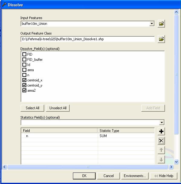
• To reduce the number of polygons choose Data Management Tools - Dissolve from the ArcToolbox and select the _union shape as input. Now select the new fields (centroid_x, centroid_y, area) as dissolve fields (to identify the identical polygons). As we are interested in the number of overlapping inclusion zones per polygon (in case that number of stems is the target), choose the field you added for the stem number as statistics field and calculate the sum:

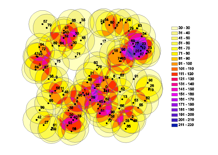
• The resulting output (_union_dissolve) should look like this if you choose a color ramp (number of classes=number of possible realizations) for the symbology:

The number of polygons in this view is the number of possible clusters of trees (and in consequence the number of different possible realizations that are derived from these clusters). In the given example a number of 200 trees with the given spatial distribution leads to a number of ~9100 possible clusters. As the target value in this example is the number of stems per ha, polygons that would lead to identical estimates if a sample point falls inside, can be classified. The number of classes is the number of possible realizations (here 1-32). The differnt colors show the inclusion area (if related to the total area this is the selection probability of a certain realization) for the different classes.

The jigsaw puzzle decomposes the infinite sample frame (infinite population approach) in an finite number of observations (finite population) whereas the area of the single polygons is expression of their selection probability. A randoml sample point would select these polygons proportional to size (PPS-sampling).

jigsaw puzzles for k-tree sampling

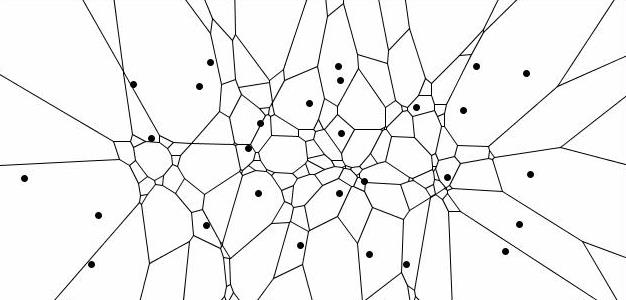
In case of k-tree sampling single trees are selected as most nearest neighbours to a sample point. In contrast to fixed area plots the neighbourhood is not defined by a maximum inclusion distance (a certain fixed bandwith) but is restricted to a fixed number of neighbours. Also in this case it is possible to create jigsaw puzzles. Same like in the example above they are a decomposition of the total domain of an infinite number of possible sample point locations in exclusive areas (polygons) for each particular realization that is possible based on the given spatial distribution of trees. Each polygon is composed by the infinite number of points that would lead to the selection of a particular cluster of k trees. The decomposition of the domain is a so called Voronoi diagramm in case of k=1 and a higher order Voronoi diagramm (kth order) in case that k neighbours are selected per sample point. The following example shows a Voronoi diagramm for 6-tree sampling.

The number of polygons is equal to the number of all possible clusters with 6 nearest trees (all points inside one polygon would select the same cluster) and as result also the number of all possible realizations of a certain target variable. The area of single polygons is, if related to the total area, an expression of the selection probability of the observation derived from the related cluster.

References

- ↑ Roesch, F.A.; Green, E.J.; Scott, C.T. 1993. An Alternative View of Forest Sampling. Survey Methodology 19 (2), 199-204.