Object-based classification (Tutorial)

Mean-shift segmentation of large size images

• Type into the search box of the Windows taskbar: mapla.bat. Click on mapla.bat to open Monteverdi Application Launcher.
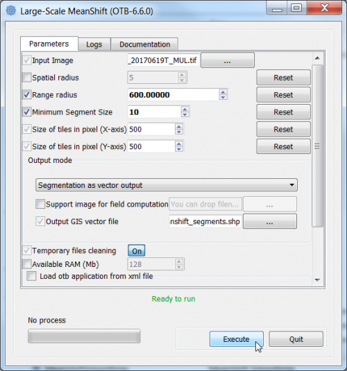
• In the search engine of mapla, type Meanshift and double click LargeScaleMeanshift.
• Select the input image: Subset_S2A_MSIL2A_20170619T_MUL.tif (datatype uint 16bits).
• The Range radius value can be set to 600. The optimal value depends on datatype dynamic range of the input image and requires experimental trials for the specific classifcation objectives.
• The value for Minimum Segment size (in pixels) can be set to 10. It depends on the size of the minimum mapping unit and the smallest object that can be destinguished.
• Leave all other configurations as they are and click Run. Have a look on the resulting filtered and spatial images.
• The Output GIS vector file is specified as a shapefile with the extension *.shp.
• Click Execute.

• Evaluate the segmentation results:

Load the output vector file into QGIS on top of the image Subset_S2A_MSIL2A_20170619T_Mul.tif Mark the vector layer in the Qgis Layers window. Layer --> Properties --> Symbology --> Simple Fill to No Brush and Stroke color to white.

Preparation of training data

• Create a dense regular point grid Vector --> Resarch tools --> Regular points... with the extent of the multispectral image and a point spacing of 200 meters.
• Install the Point sampling plugin.
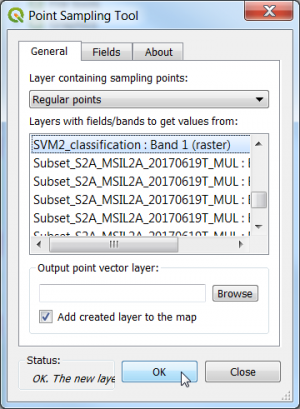
• Extract the landcover class from an existing thematic classifcation map using the Point Sampling Tool.

.

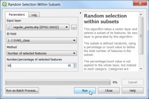
• Select 50 points in each class stratified sampling with equal allocation: Vector --> Resarch tools --> Random section within subsets....

.

• Join the Land use/cover (LUC) class attribute of previous digitized training area polygons with the image segments. Vector --> Data Management Tools --> Join Attributes by Location ....

1. 1. • The Target vector file is the Output GIS vector file of step 4.
      • Join vector layer is training_manual_poly.shp.
      • Output vector seg_Subset_S2A_MSIL2A_20170619T_BOA_train.shp.
      • For the rest of parameters keep default values.OK.

Rename the field names of the resulting output vector attribut table avoiding upper capitals and underline using the Table Manager plugin. Rename the attribut field C_ID to class.

Object-based classifcation using SVM algorithm

We may use the windows command line and OTB QT graphical user interfaces. Start --> All Programs --> OSGeo4W --> OSGeo4W Shell or double click on the file C:\OSGeo4W64\OSGeo4W.bat.

1. A windows command shell opens, please type otbgui_ComputeOGRLayersFeaturesStatistics.
   1. • Name of the input vector is seg_Subset_S2A_MSIL2A_20170619T_BOA_train.shp.
      • XML file containing mean and variance of each feature is seg_Subset_S2A_MSIL2A_20170619T_BOA_train.xml.
      • In the List of features to consider for statistics mark the columns meanB0, meanB1, meanB2.Execute. Calculate also an XML file for vector file seg_Subset_S2A_MSIL2A_20170619T_BOA.shp.
2. Type into the OSGeo4W shell otbgui_TrainOGRLayersClassifier.
   1. • Name of the input shapefile is seg_Subset_S2A_MSIL2A_20170619T_BOA_train.shp.
      • XML file containing mean and variance of each feature is seg_Subset_S2A_MSIL2A_20170619T_BOA_train.xml.
      • Output model filename is seg_Subset_S2A_MSIL2A_20170619T_BOA_train.model
      • In the List of features to consider for statistics mark the columns meanB0, meanB1, meanB2, ...
      • The name ofField containing the class id for supervision" is class.Execute.
3. Type into the OSGeo4W shell otbgui_OGRLayerClassifier.
   1. • Name of the input shapefile is seg_Subset_S2A_MSIL2A_20170619T_BOA.shp.
      • XML file containing mean and variance of each feature is seg_Subset_S2A_MSIL2A_20170619T_BOA.xml.
      • Input model filename is seg_Subset_S2A_MSIL2A_20170619T_BOA_train.model
      • In the List of features to consider for statistics mark the columns meanB0, meanB1, meanB2, ...
      • The name ofField containing the predicted class" is predicted.Execute.
4. Open the resulting vector file in a QGIS map view.
   1. • Change the style of the classified vector layer: Go to layer properties --> style. Click on ‘Load Style’. Browse for OBIA_legend file and select OBIA_legend.qml}}. apply, OK.
5. Simplify the vector file using Vector --> Geoprocessing Tools --> Dissolve...
   1. • Input vector layer is seg_Subset_S2A_MSIL2A_20170619T_BOA.shp.
      • Dissolve field is predicted.
      • Output shapefile is seg_188_Subset_S2A_MSIL2A_20170619T_BOA_diss.shp

Info

For more detailed information on the SVM algorithm visit the library website