Adaptive cluster sampling
{Language}
Contents |
Introduction
There are target objects in forest inventory which are rare, such as rare tree or shrub species. They are sparsely distributed over the population of interest and using the usual sampling designs will face the situation that most of the plots are empty and then there are some few plots with the objects of interest. Here, one of the problematic features becomes obvious: in design-based statistical sampling we do only observe and record what is there on the sample plot (Kleinn 2007[1]). Nothing else. Outside the observation plot we pretend to be blind; and so we do on the some times long way to the sample plot! It is hypothesized that this is a waste of resources and that there must be sound ways of including such additional observations / information into a design-based estimation.
Sampling for rare events is a science in itself and there are whole textbooks about that specific topic. Often, the simplest solution is to increase sample size in order to increase the probability to encounter the rare objects; however, this increases travel cost and labor cost as well.
If it is known or suspected for some reasons that the rare species forms clusters or groups within the population of interest, then, one may be interested to establish plots around the sampled plot once a sampled plots contains a rare element; because then, one would expect more elements around that plot. The sampling strategy, that implies enlarging the plot once a target element is found on the initial plot, is called Adaptive Cluster Sampling (ACS). In general, adaptive samplings are sampling strategies that adapt to specific situations. That means, that the final design that is implemented (in the field) is not completely predictable but depends also on what is being found out there. This conditional adaptation of the design makes estimation difficult, because the selection probability is then obviously a conditional probability. And the selection probability of a specific element depends also on the proximity of other elements,
Just like cluster sampling, neither adaptive cluster sampling is, strictly spoken, a sampling design by its own, it is a variation of response design in which the plot size adapts to the specific situation found in the field. For this adaptation, however, clear rules need to be defined.
Adaptive cluster sampling has been developed and introduced by Thompson (Thompson 1992[2]); he is also the author of a textbook on the more general approach of adaptive sampling (Thompson and Seber 1996[3]). Our presentation of adaptive cluster sampling here follows his publications. Adaptive cluster sampling is relatively frequently applied in research studies; application in “production forest inventories” is very rare, however, if any!
General procedure
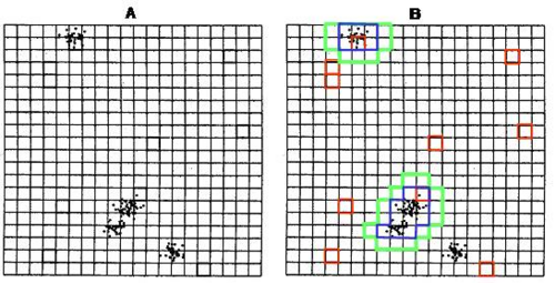
In Step 1, a random sample of \(n\) plots is selected; this is some times called the initial sample or the seed sample. In Step 2, for each initial plot, we determine whether the target element is there or not; or in general terms: whether the specified condition is fulfilled or not. If the condition is fulfilled (for example: there is at least one of the target species on that initial plot), then all its neighboring plots are also observed. Then again, neighbors of these new plots (that are now sub-plots, actually) will be observed if the plots fulfill the specified condition. This procedure is continued until no more plots are found at the periphery of the cluster of sub-plots that fulfill the condition. By this procedure, the plot design adapts to the situation encountered in the field. Clusters of sub-plots are generated by this procedure which are irregular in shape and unequal in size. It is the occurrence of the objects of interest that defines the final shape and size of the clusters. However, the number of clusters is determined by the initial sample (if not neighboring clusters grow together).
The above picture shows an application of standard adaptive cluster sampling as developed by Thompson. The left graph shows the population of clustered and relatively rare events, thus the population of interest. In the right graph, the adaptive clustering process is depicted: the red squares are the randomly selected \(n\) initial plots (Thompson 1992). The green depicts the clusters that are eventually expanded according to a specific rule, while the blue plots are the sets of plots surrounding the initial sampled plot and satisfying the specific rule.
Terminology
Some terms need to be defined in the context of adaptive cluster sampling:
- Cluster: a set of plots around the sampled plot, which is the final result of the selection along the defined adaptation procedure.
- Network: a subset of all plots within a cluster such that if any plot of the network is selected, all other plots of this network will enter into the sample.
- Edge: neighboring plots of a network. Selecting an edge plot does not make an additional plot enter the sample. However, if a network is selected to be in the sample, its edge plots will enter the sample as a ring around the network.
- If there is a plot that does not fulfill the specific condition, it is defined as a network of size 1. This implies that the population is composed of networks, and we can specify the selection probability for each network.
Selection probabilities
In adaptive cluster sampling, the probability of selecting a plot depends on both the sampling design and the structure of the population. Therefore, the selection probability is not the same for all sample elements.
There are two possibilities of a plot \(i\) to enter the sample: either if any plot of the network to which the plot belongs is selected in the initial sample including plot \(i\) by itself or if a network is selected to which plot \(i\) is an edge.
Let \(m_i\) be the size of the network to which plot \(i\) belongs to, and \(a_i\) the total number of plots in the networks to which plot \(i\) is an edge. Then, if \(i\) fulfills the condition to extend the plot, then, \(i\) is not an edge, \(a_i=0\); else, \(m_i=1\), where \(i\) is an edge or plot that does not lead to extension.
The selection probability in one draw is
\(P_i=\frac{m_i+a}{N}\,\),
and the inclusion probability of \(n\) draws with replacement is
\(\pi_i=1-(1-P_i)^n\,\),
and without replacement,
\(\pi_i=1-\frac{\left(\begin{matrix}N-m_i-a_i\\n\end{matrix}\right)}{\binom{N\,}{n\,}}\,\).
Estimators
The adaptive enlargement of field clusters can be applied to any of the basic sampling techniques. The estimators in this section refer to simple random sampling of initial plots only. For other sampling techniques, appropriate estimators have to be looked up or developed.
In adaptive cluster sampling, each network is viewed as one independent observation. Each network can, therefore, be viewed as a one cluster, where the clusters are irregular in shape an unequal in size. We may imagine the sampling process then as simple random sampling of clusters where clusters are of unequal size: either a network of size 1 is selected (an “empty” cell) or the initial sample hits a “full” cell (which satisfies the specified condition) and then the entire cluster is automatically selected.
The mean of the observations in network \(i\) which has been selected into the sample is
\(w_i=\frac{1}{m_i}\sum_{j\epsilon\psi}y_j\,\), where, \(\psi_i\,\)
is the plots in network \(I\), which in fact should be named sub-plots as they are components of the entire cluster-plot!
The mean of all networks in the sample results then as usual from
\(\bar y_i=\frac{1}{n}\sum_{i=1}^n w_i\,\),
so that the parametric variance of the mean without replacement is
\(var(\bar y_i)=\frac{N-n}{N-1}\frac{1}{n}\frac{\sum_{i=1}^n\left(w_i-\mu\right)^2}{N}\,\),
and the estimated variance of the mean without replacement
\(\hat {var}(\bar y_i)=\frac{N-n}{N}\frac{1}{n}\frac{\sum_{i=1}^n\left(w_i-\bar y_i\right)^2}{n-1} \,\).
For sampling with replacement, the parametric variance of the mean is
\(\hat{var}(\bar y_i)=\frac{1}{n}\frac{\sum_{i=1}^n\left(w_i-\mu\right)^2}{N}\,\)
and the sample based estimated variance
\(\hat{var}(\hat y_i)=\frac{1}{n}\frac{\sum_{i=1}^n\left(w_i-\bar y_i\right)^2}{n-1}\,\).
Thompson (1992) elaborates on these estimators and many more in more detail.
Characteristics of adaptive cluster sampling
The practical and statistical performance of adaptive cluster sampling depends on the structure of population as the cluster plot adapts to specific conditions. If the target objects elements do not form grouping or clustering, then, there is no real advantage in applying adaptive cluster sampling.
If, however, the target objects in the population come in clusters, then we collect more information by adaptive cluster sampling, simply because we assure that larger plots are included than in the initial sample and these larger plots contain more data of those target objects.
If we look at it in terms of spatial autocorrelation as discussed with cluster sampling, however, we may expect relatively high intra-cluster correlation because we are always include the immediate neighbor plots to the initial plots selected; and the immediate neighbors may be expected to exhibit considerable correlation because of the small distance. Therefore, it may be that we observe more target objects but we do not add much additional independent information by expanding the clusters; this would be a statistical argument not in favor of adaptive cluster sampling.
From a practical perspective, it is, of course, more work to lay out a network of square plots rather than measuring simple initial plots only; and this should be justified by an increase in statistical precision.
If the objective of a sampling study is to observe more of rare target objects than would be observed in standard sampling, then adaptive cluster sampling has a clear advantage if the target objects occur in clusters. It is obvious, that we will not expect any superiority if the rare events are scattered individually over the area of interest, as there would hardly be any plot that would be enlarged beyond the initial size of the plot.
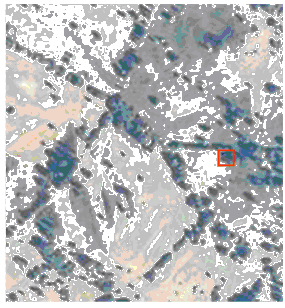
However, there are also populations with a spatial structure of clustering which poses a certain problem to adaptive cluster sampling, for example when sampling for trees outside the forest (see figure on the right side). This tree resource is of increasing interest also in the context of carbon sequestration projects. Trees outside the forest are usually relatively rare events that come in any spatial arrangement: as isolated individual trees, as blocks of trees and also frequently in lines (live fences, alleys etc.). In that case, when attempting to apply adaptive cluster sampling we will run rapidly into the situation that the clusters become unacceptably large (of course, that may happen with any large cluster, not only with trees in lines!).
In such cases, a so-called cut-off rule need to be used, defining that the adaptive enlargement of the cluster is finished after a defined maximum cluster size is reached. That makes estimation more complex.
 Adaptive cluster sampling examples: Examples for Adaptive cluster sampling
References
- ↑ Kleinn, C. 2007. Lecture Notes for the Teaching Module Forest Inventory. Department of Forest Inventory and Remote Sensing. Faculty of Forest Science and Forest Ecology, Georg-August-Universität Göttingen. 164 S.
- ↑ Thompson SK. 1992. Sampling. John Wiley & Sons. 343 p.
- ↑ Thompson SK and GAF Seber. 1996. Adaptive Sampling. 1996. John Wiley & Sons, Wiley Series in PRobability and Statstics. 256 p.

