Variance issue in systematic sampling

Languages:

English

Forest Inventory lecturenotes

Category Forest Inventory lecturenotes not found

Empirical approximation of error variance

Again and again: there is no design-unbiased variance estimator in systematic sampling. If we are interested in the true error variance, the only way is to very often repeat the systematic sample and calculate the variance of all the estimations produced; that is then an empirical approximation to the parametric error variance which is the closer to the unknown true value the larger the number of repetitions is. Of course, this is not a viable approach for practical implementation, but it is something that can be done in computer simulations.

Using SRS estimators

What is most frequently done for variance estimation in systematic sampling is that the simple random sampling framework of estimators is applied. It is clear and known that these estimators are not unbiased for systematic sampling but they yield consistently over-estimations of the true error variance; this positive bias can be considerable. We call this sort of estimation a “conservative estimation”: we know that the true error is less (in many cases much less) than the estimation that has been calculated. An example is presented further down in the article Area estimation by points, where the area estimation by dot grids is presented.

Remember

For error variance estimation we use to apply the simple random sampling estimator

\(s_\bar y^2=\frac{s^2}{n}\)

(essentially, because we do not \(k\) now better …). This, however, is not an unbiased estimator but produces an overestimation of the true error variance.

Random differences method

Numerous approximations had been developed to better approximate the true error variance than with the simple random sampling estimator. Two of the more simple ones are presented here, starting with the so called “random differences method”.

Assume that the elements in the population and also the \(n\) elements that are in the systematic sample have the same expected value. We actually may assume that because we have an unbiased estimator for the mean. If we select (repeatedly) random pairs out of the \(n\) elements of the systematic sample and calculate the difference for each of the pairs, we would expect the expected value of this difference to be zero:

Let \(d\) be \(Y_1-Y_2\), then \(E(d)=\mu=E(Y_1-Y_2)=E(Y_1)-E(Y_2)=0\).

The variance of the difference \(var(\bar d)=var(Y_1-Y_2)\) is then be determined along the rules for linear combinations of random variables as known from developing the estimators for stratified random sampling; as we select each one of the two elements of a pair independently at random, the covariance term below becomes zero:

\(var(\bar d)\)	\(=var(Y_1-Y_2)\,\)
	\(=var(Y_1)+var(Y_2)-2cov(Y_1Y_2)\,\)
	\(=var(Y_1)+var(Y_2)\,\)
	\(=2\sigma^2\,\)

where \(\sigma^2\) is the population variance of both \(Y1\) and \(Y2\), which is the same. If \(n_d\) pairs are formed, that population variance \(\sigma^2\) is estimated by

\(2\sigma^2=\frac{\sum_{i=1}^{n_c}\left(d_i-\bar{d}\right)^2}{n_d}=\frac{\sum_{i=1}^{n_d}d_i^2}{n_d}\,\)

and the estimated error variance of the mean for systematic sampling with the random pairs method is

\(\hat{var_{rd}}\left(\bar y_{syst}\right)=\frac{\hat{\sigma}^2}{n}=\frac{1}{n}\frac{1}{2n_d}\sum_{i=1}^{n_d}d_i^2\,\).

Pair difference technique

Figure 1 Building pairs of neighboring observations for the approximation of error variance in systematic sampling (Kleinn 2007). Pairs can either be built “exclusively” (below) or overlapping (above).

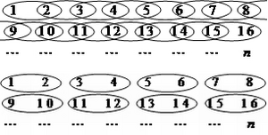
Another approach had been developed by Lindeberg (1924) analyzing the systematic field data of the early Nordic national forest inventories. He imagined neighboring observations to form a stratum so that the whole sample of \(n\) elements consists of \(n/2\) strata and in each stratum the sample size is \(n_h = 2\) (see Figure 1). Then, he applied the formula for stratified random sampling and came up with the below formula. Of course, this is again only an approximation because neither the estimators of stratified random sampling apply, because sampling within the strata was not random.

However, it proved in many simulation studies that this approximation is in many cases fairly close to the true error variance; some times over-estimating, some times under-estimating; depending on the population structure and the sample taken. An example for area estimation with dot grids is presented in the chapter "Comparison of different grid shapes in systematic sampling", which can be found below.

In a stratum with \(n_h=2\) elements randomly sampled, the population variance within that stratum \(h\) is estimated from

\(s_h^2=\frac{\sum_{i=1}^n\left(y_{hi}-\bar{y}_h\right)^2}{n_h-1}=\frac{1}{2}\left(y_{h1}-y_{h2}\right)^2\,\)

- where the variance formula converts into a simple squared difference.

Assuming that we form \(L\) strata of the same size so that the stratum weights are constantly \(w_h=1/L\). The error variance for the total of all strata results then as usual in stratified random sampling from

\(\hat{var}_{pd}\left(\bar{y}_{syst}\right)=\sum_{h=1}^L w_h^2\frac{s_h^2}{n_h}=\sum_{h=1}^L\frac{\left(y_1-y_2\right)^2}{4L^2}\,\).

This estimation corresponds actually to the error variance estimator of the random differences technique if we select \(n_d=n/2\) pairs of observations:

\(\hat{var}_{rd}\left(\bar{y}_{syst}\right)\,\)	\(=\frac{1}{n}\frac{1}{2n_d}\sum_{i=1}^{n_d}d_i^2\,\)
	\(=\frac{1}{2n_d}\frac{1}{2n_d}\sum_{i=1}^{n_d}d_i^2\,\)
	\(=\frac{1}{4L^2}\sum_{i=1}^{n_d}d_i^2\,\)

The pair differences technique may also be applied for overlapping pairs as depicted in Figure 1.

Pair difference technique example: Example for Pair difference technique

References

sorry:

This section is still under construction! This article was last modified on 12/23/2010. If you have comments please use the Discussion page or contribute to the article!

References

- ↑ Kleinn, C. 2007. Lecture Notes for the Teaching Module Forest Inventory. Department of Forest Inventory and Remote Sensing. Faculty of Forest Science and Forest Ecology, Georg-August-Universität Göttingen. 164 S.