Fixed area plots
From AWF-Wiki
(Difference between revisions)
(→Nested sub-plots) |
(→General observations) |
||
| Line 6: | Line 6: | ||
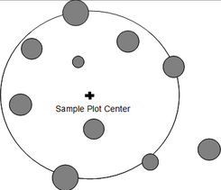
[[File:4.2.2-fig46.png|right|thumb|245px|'''Figure 1''' With circular sample plots all trees are taken as sample trees that are within a defined distance (radius) from the sample point, which constitutes the plot center (Kleinn 2007<ref name="kleinn2007">Kleinn, C. 2007. Lecture Notes for the Teaching Module Forest Inventory. Department of Forest Inventory and Remote Sensing. Faculty of Forest Science and Forest Ecology, Georg-August-Universität Göttingen. 164 S.</ref>).]] | [[File:4.2.2-fig46.png|right|thumb|245px|'''Figure 1''' With circular sample plots all trees are taken as sample trees that are within a defined distance (radius) from the sample point, which constitutes the plot center (Kleinn 2007<ref name="kleinn2007">Kleinn, C. 2007. Lecture Notes for the Teaching Module Forest Inventory. Department of Forest Inventory and Remote Sensing. Faculty of Forest Science and Forest Ecology, Georg-August-Universität Göttingen. 164 S.</ref>).]] | ||
| − | [[File:4.2.2-fig47.png|right|thumb|245px|'''Figure | + | [[File:4.2.2-fig47.png|right|thumb|245px|'''Figure 2''' Illustration of the inclusion zone approach: For fixed area circular plots, the inclusion zones are identical for all trees. Those trees are taken as sample trees in whose inclusion zones the sample point comes to lie (Kleinn 2007<ref name="kleinn2007">Kleinn, C. 2007. Lecture Notes for the Teaching Module Forest Inventory. Department of Forest Inventory and Remote Sensing. Faculty of Forest Science and Forest Ecology, Georg-August-Universität Göttingen. 164 S.</ref>).]] |
| + | [[File:4.2.2-fig48.png|right|thumb|245px|'''Figure 3''' Typical diameter distribution in a natural forest (Kleinn 2007<ref name="kleinn2007">Kleinn, C. 2007. Lecture Notes for the Teaching Module Forest Inventory. Department of Forest Inventory and Remote Sensing. Faculty of Forest Science and Forest Ecology, Georg-August-Universität Göttingen. 164 S.</ref>).]] | ||
| + | [[File:4.2.2-fig49.png|right|thumb|245px|'''Figure 4''' Nested sub-plots showing 3 circular plots having different sizes, radii, but sharing same plot center (Kleinn 2007<ref name="kleinn2007">Kleinn, C. 2007. Lecture Notes for the Teaching Module Forest Inventory. Department of Forest Inventory and Remote Sensing. Faculty of Forest Science and Forest Ecology, Georg-August-Universität Göttingen. 164 S.</ref>).]] | ||
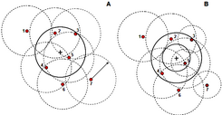
| + | [[File:4.2.2-fig50.png|right|thumb|245px|'''Figure 5''' Comparison of the inclu-sion zone approach for nested circular sub-plots (B) and for fixed circu-lar plots (A) (Kleinn 2007<ref name="kleinn2007">Kleinn, C. 2007. Lecture Notes for the Teaching Module Forest Inventory. Department of Forest Inventory and Remote Sensing. Faculty of Forest Science and Forest Ecology, Georg-August-Universität Göttingen. 164 S.</ref>).]] | ||
| + | [[File:4.2.2-fig51.png|right|thumb|245px|'''Figure 6''' Different combination of shapes for nested sub-plots (after Prodan et al. 1997<ref name="prodan1997">Prodan M., R. Peters, F. Cox and P. Real 1997. Mensura forestal. Serie investigación y educación en desarrollo sostenible. IICA/GTZ. 561p.<ref>.]] | ||
Fixed area sample [[Sampling design and plot design|plots]] can have various different shapes including circular, square, rectangular and strip. As to which shape is chosen depends on practical and statistical issues. In terms of practical criteria it is mainly the cost which is of interest and which translates into criteria such as terrain conditions and expected frequency of border [[Tree Definition|trees]]. Border trees cost time because it needs to be carefully checked whether they are in or not and that implies usually additional [[Distance to tree|distance]] measurements which are not required for the other trees. | Fixed area sample [[Sampling design and plot design|plots]] can have various different shapes including circular, square, rectangular and strip. As to which shape is chosen depends on practical and statistical issues. In terms of practical criteria it is mainly the cost which is of interest and which translates into criteria such as terrain conditions and expected frequency of border [[Tree Definition|trees]]. Border trees cost time because it needs to be carefully checked whether they are in or not and that implies usually additional [[Distance to tree|distance]] measurements which are not required for the other trees. | ||
| + | |||
From a practical point of view a circular plots is most rapidly installed wherever the visibility in the stand is good. In a tropical forest with dense understory, it is much easier to establish a strip plot where the field crew walks along the central line and measures all trees up to a defined distance to the right and to the left. A circular plot, however, has the lowest expected number of border trees, because, for a given area, the circle is the geometric shape that has the shortest perimeter. | From a practical point of view a circular plots is most rapidly installed wherever the visibility in the stand is good. In a tropical forest with dense understory, it is much easier to establish a strip plot where the field crew walks along the central line and measures all trees up to a defined distance to the right and to the left. A circular plot, however, has the lowest expected number of border trees, because, for a given area, the circle is the geometric shape that has the shortest perimeter. | ||
From a practical point of view, coming back to the considerations on [[Introduction to plot design#Spatial autocorrelation|spatial autocorrelation]], a long rectangular plot (strip plot) covers more different site conditions and is likely to capture more variability per plot. Thus, we may expect higher precision when using strip plots if we compare it with circular plots with the same plot area. | From a practical point of view, coming back to the considerations on [[Introduction to plot design#Spatial autocorrelation|spatial autocorrelation]], a long rectangular plot (strip plot) covers more different site conditions and is likely to capture more variability per plot. Thus, we may expect higher precision when using strip plots if we compare it with circular plots with the same plot area. | ||
| + | |||
In what refers to the plot size, for a given sampling intensity it is statistically more precise to establish many small plots than few large plots. However, with many small plots, again the cost will be much higher; the decision on [[Sample size|plot size]] is again a compromise between practical (cost) criteria and statistical (precision). If there is some information on number of stems per hectare, one can calculate, as a rule of thumb, the plot area such that there are on average about 15-20 trees in a sample plot. Typical plot areas are 200 m², 500 m², 1000 m² - but anything is possible. | In what refers to the plot size, for a given sampling intensity it is statistically more precise to establish many small plots than few large plots. However, with many small plots, again the cost will be much higher; the decision on [[Sample size|plot size]] is again a compromise between practical (cost) criteria and statistical (precision). If there is some information on number of stems per hectare, one can calculate, as a rule of thumb, the plot area such that there are on average about 15-20 trees in a sample plot. Typical plot areas are 200 m², 500 m², 1000 m² - but anything is possible. | ||
Revision as of 07:47, 3 March 2011
| sorry: |
This section is still under construction! This article was last modified on 03/3/2011. If you have comments please use the Discussion page or contribute to the article! |
Forest Inventory lecturenotes
Category Forest Inventory lecturenotes not found
Contents |
General observations

Figure 1 With circular sample plots all trees are taken as sample trees that are within a defined distance (radius) from the sample point, which constitutes the plot center (Kleinn 2007[1]).

Figure 2 Illustration of the inclusion zone approach: For fixed area circular plots, the inclusion zones are identical for all trees. Those trees are taken as sample trees in whose inclusion zones the sample point comes to lie (Kleinn 2007[1]).

Figure 3 Typical diameter distribution in a natural forest (Kleinn 2007[1]).

Figure 4 Nested sub-plots showing 3 circular plots having different sizes, radii, but sharing same plot center (Kleinn 2007[1]).

Figure 5 Comparison of the inclu-sion zone approach for nested circular sub-plots (B) and for fixed circu-lar plots (A) (Kleinn 2007[1]).
[[File:4.2.2-fig51.png|right|thumb|245px|Figure 6 Different combination of shapes for nested sub-plots (after Prodan et al. 1997Cite error: Closing </ref> missing for <ref> tag
Cite error:
<ref> tags exist, but no <references/> tag was found