Ratio estimator sampling examples

Revision as of 12:22, 18 January 2011

Example 1:

Figure 1 Example of a population of 30 unequally sized strip plots; here, the ratio estimator may be applied for estimation using plot size as co-variable (DeVries 1986^[1]).

Recall \(k\)-tree sampling as presented and discussed in distance based plots. One approximation to estimation is to imagine a virtual circle plot through the \(k^{th}\) tree, that is, a circle which has a radius that corresponds to the distance between the sample point and the \(k^{th}\) tree. Depending on the distance to the \(k^{th}\) tree, these circle plots will have very different sizes: in parts of the forest with a high stem density, the plots will be small and in low density sectors, the plots will be large.

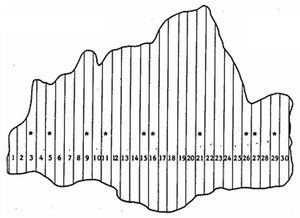
It is some times suggested to use the ratio estimator to cope for this unequal plot sizes, just as we suggested it for the above case of unequally sized strip plots (Figure 1).

However, why is this not a good idea?

Recall what we said about the situations in which the ratio estimator is efficient: a high positive correlation between target variable and ancillary variable needs to be present. In our case, number of stems could be a target variable and plot size the ancillary variable. It can directly be seen without any calculations that the correlation is zero: the number of stems is constant \((k)\) and thus completely uncorrelated with plot area – it is always the same.

Therefore, application of the ratio estimator to improve precision of the empirical \(k\)-tree sampling estimators is useless.

Example 2:

Lets take the example population as of Figure 1.

At first, we calculate the parametric values: the totals are \(\tau_X=4185\) units of area, and \(\tau_Y=212m^3\), if we take the value of the target variable as growing stock in \(m^3\) for the time being. Parametric means are \(\mu_X=193.5\) area units and \(\mu_Y=7.067m^3\) for ancillary and target variable, respectively; and the parametric variances in the population are

\[{\sigma_x}^2=2087.25\]

and

\[{\sigma_y}^2=7.13\].

The parametric correlation is \(\rho=0.8815\) and the true ratio

\[R=\frac{\mu_Y}{\mu_X}=\frac{\sum_{i=1}^N y_i}{\sum_{i=1}^N x_i}=0.050657\,\].

Again: all these values are parametric values that can only be calculated if the population is known; these values are unknown when real sampling studies are carried out. Here, we use them as reference.

Now let’s calculate the parametric variances of the estimated mean first for the ratio estimator and then for comparison, for the simple random sampling estimator. The latter had been calculated earlier: the parametric variance of the estimated mean (simple random sampling) is

\[var(\bar{y})=0.4916=\frac{fpc*{\sigma_Y}^2}{n}\,\]

and the error variance of the estimated total

\[var(\hat\tau)=N^2*var(\bar y)=900*0.4917=442.48\,\].

For the ratio estimator, the parametric value of the error variance of the estimated mean is

\[var(\bar y)=\frac{N-n}{N-1}\frac{1}{n}\left\{{\sigma_y}^2+R^2{\sigma_x}^2-2R\rho\sigma_x\sigma_y\right\}=0.109684\,\]

and the error variance of the estimated total

\[var(\hat \tau)=var(\bar y)*30^2=98.7154\,\].

In this case, we see that – due to the high positive correlation – the ratio estimator produces much more precise estimations. The parametric error variance for the estimated mean is with 0.109684 only about one forth to one fifth of the error variance that the simple random sampling estimator produced. In other words: by using the ratio estimator with plot area as ancillary variable, one needs much less samples (and, therefore, resources, to achieve a defined precision).

We may quantify this superiority by calculating the relative efficiency

\[RE=\frac{var\left(\bar{y}_{random}\right)}{var\left(\bar{y}_{ratio}\right)}=\frac{0.4917}{0.1097}=4,48\,\];

that is: the ratio estimator is 4.48 times as efficient as the simple random sampling estimator, in this particular example.

We may also use the inequality presented in the article Ratio Estimator: Efficiency to know that the ratio estimator is superior:

\[\rho\ge\frac{R\sigma_x}{s\sigma_y}=\frac{cv(x)}{2cv(y)}\,\].

In the present example, we have

\[0.8816\ge^{??}\frac{0.0507*445.69}{2*2.67}=\frac{0.3275}{2*0.3778}=0.4334\,\]

and we see that the parametric correlation present in the population is clearly larger than the calculated minimum value of 0.4334.

References

1. ↑ de Vries, P.G., 1986. Sampling Theory for Forest Inventory. A Teach-Yourself Course. Springer. 399 p.