Revision as of 13:15, 16 December 2020

Object-based image analysis (OBIA) with QGIS and OTB processing plugin

Segmentation

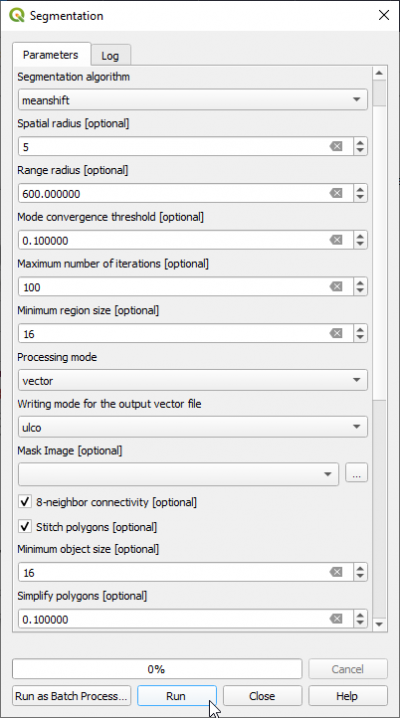
• In the search engine of Processing Toolbox, type segmentation and double click Segmentation.
• Set Segmentation algorithm to meanshift
• Select the input image: Subset_S2A_MSIL2A_20170619T_MUL.tif (data type uint 16bit).
• The Range radius value can be set to 600. The optimal value depends on datatype dynamic range of the input image and requires experimental trials for the specific classifcation objectives.
• Set Minimum Region size (in pixels) to 16.
• Processing mode Vector
• Set the Mask image to blank (top of dro-down list).
• The Minimum Segment size (in pixels) can be set to 16 depending on minimum mapping size.
• Check 8-neighborhood connectivity on.
• Change Output pixel type to uint32.
• Name the Output vector file e.g. lucc_meanshift_seg.gpkg (GeoPackage).
• Click Run.

• Evaluate the segmentation results: Load the output vector file lucc_meanshift_seg.shp into QGIS on top of the image Subset_S2A_MSIL2A_20170619T_Mul.tif

Mark the vector layer in the Qgis Layers window. Layer --> Properties --> Symbology --> Simple Fill, Fill Style: No Brush and Stroke color:white.

Feature extraction

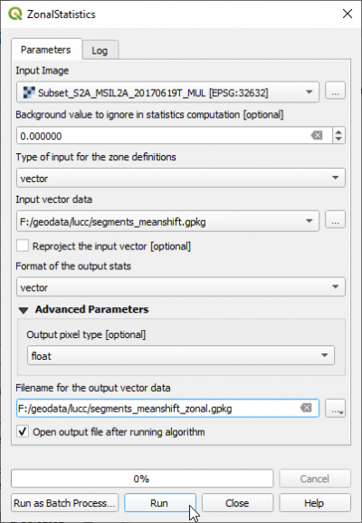
Since OTB 7.0.0: In the search engine of Processing Toolbox, type zonalstats and open ZonalStatistics under Image Manipulation of OTB.

• Select the Input image: Subset_S2A_MSIL2A_20170619T_MUL.tif .
• Background value to ignore: 65535
• The input vector data is the result from Segmentation: lucc_meanshift_seg.shp.
• File name for the output vector data: lucc_meanshift_seg_stats.shp.
• File name for the raster image: lucc_meanshift_seg_stats.tif. (not necessary in vector processing mode but still a bug in QGIS 3.10).
• Click Run.

Alternative module:

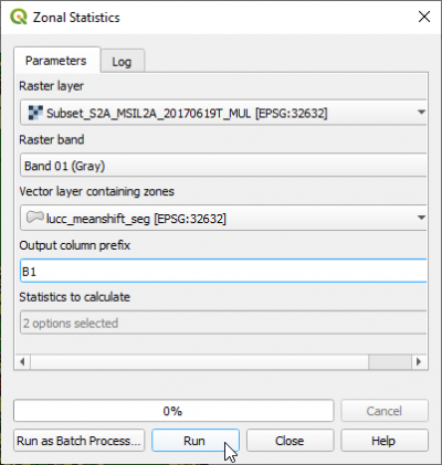
• In the search engine of Processing Toolbox, type zonal and double click Zonal Statistics.
• Select the Raster layer: Subset_S2A_MSIL2A_20170619T_MUL.tif .
• Set Raster band Band 01.
• The vector layer containing zones is the result from Segmentation: lucc_meanshift_seg.shp.
• Change output column prefix to the original Sentinel-2 band name: B1
• In the list Statistics to calculate just check two measures: Mean and Std. dev..
• Click Run.

• Repeat the procedure for bands 02, 03, 04, 05, 06, 07, 08, 09, 10.
• Open the attribute table of vector layer lucc_meanshift_seg.shp containing now statistics for each zone or segment.

Training phase

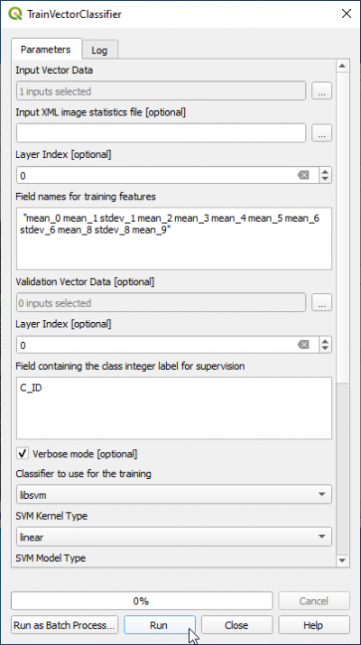
• In the search engine of Processing Toolbox, type Train and double click TrainVectorClassifier.
• Name of the input shapefile is train_input_OBIA.shp.
• Output model filename is lucc_svm_obia.model
• In the field Field names for training features copy and paste

for OTB 7.0.0 Zonalstatistics module:

 "mean_0 mean_1 stdev_1 mean_2 mean_3 mean_4 mean_5 mean_6 stdev_6 mean_8 stdev_8 mean_9" 

or if you used the qgis zonal statistics module:

 "B1mean B2mean B2stdev B3mean B4mean B5mean B6mean B7mean B7stdev B9mean B9stdev B10mean" 

• The name of Field containing the class id for supervision" is C_ID.
• Classifier to use for training: libsvm
• SVM Kernel Type: linear
• SVM Model Type: csvc
• Click Parameters optimizationON.
• Click Run.

Info

For more detailed information on the SVM algorithm visit the LibSVM website

Classification phase

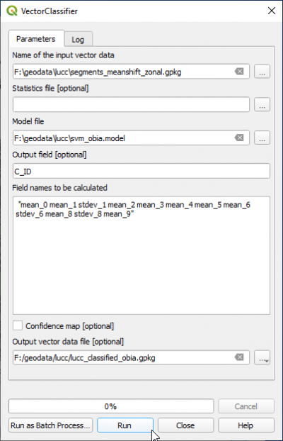
• In the search engine of Processing Toolbox, type Vector and double click VectorClassifier.
• Name of the input vector data is lucc_segments.shp.
• Name of the input model file is lucc_svm_obia.model.
• Output field containing the class is C_ID
• Copy and paste into the filed Field names to be calculated the same features as in the TrainVectorClassifier module:

for OTB 7.0.0 Zonalstatistics module:

 "mean_0 mean_1 stdev_1 mean_2 mean_3 mean_4 mean_5 mean_6 stdev_6 mean_8 stdev_8 mean_9" 

or if you used the qgis zonal statistics module:

 "B1mean B2mean B2stdev B3mean B4mean B5mean B6mean B7mean B7stdev B9mean B9stdev B10mean" 

• Specify the Output vector file. Run

Object-based image analysis (OBIA) with OTB standalone

Segmentation

• Type into the search box of the Windows taskbar: mapla.bat. Click on mapla.bat to open Monteverdi Application Launcher.
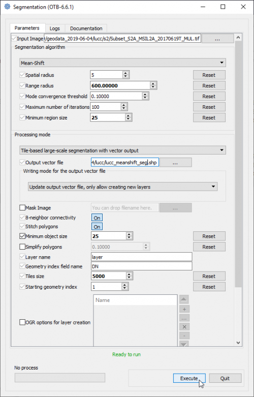
• In the search engine of mapla, type Segmentation and double click Segmentation.
• Select the input image: Subset_S2A_MSIL2A_20170619T_MUL.tif (datatype uint 16bits).
• The Range radius value can be set to 600. The optimal value depends on datatype dynamic range of the input image and requires experimental trials for the specific classifcation objectives.
• The value for Minimum Segment size (in pixels) can be set to 25. It depends on the size of the minimum mapping unit and the smallest object that can be destinguished.
• Leave all other configurations as they are and click Run. Have a look on the resulting filtered and spatial images.
• The Output GIS vector file is specified as a shapefile with the extension *.shp.
• Click Execute.

• Evaluate the segmentation results:

Load the output vector file into QGIS on top of the image Subset_S2A_MSIL2A_20170619T_Mul.tif Mark the vector layer in the Qgis Layers window. Layer --> Properties --> Symbology --> Simple Fill to No Brush and Stroke color to white.

Info

For more detailed information on the SVM algorithm visit the LibSVM website

Feature extraction

• In the search engine of Processing Toolbox, type zonal and double click Zonal Statistics.
• Select the Raster layer: Subset_S2A_MSIL2A_20170619T_MUL.tif .
• Set Raster band Band 01.
• The vector layer containing zones is the result from Segmentation: lucc_meanshift_seg.tif.
• Change output column prefix to the original Sentinel-2 band name: B1
• In the list Statistics to calculate just check two measures: Mean and Std. dev..
• Click Run.

• Repeat the procedure for bands 02, 03, 04, 05, 06, 07, 08, 09 and 10.
• Open the attribute table of vector layer lucc_meanshift_seg.tif containing now statistics for each zone or segment.

Training phase

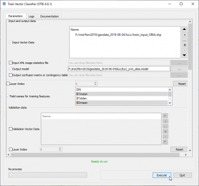
• In the search engine of mapla, type Train and double click TrainVectorClassifier.
• Name of the input shapefile is train_input_OBIA.shp.
• Output model filename is lucc_svm_obia.model
• In the list Field names for training featrues mark 11 columns: B1mean, B2mean, B2stdev, B3mean, B4mean, B5mean, B6mean, B7mean, B7stdev, B9mean, B9stdev, B10mean with Ctrl + left-click.
• The name of Field containing the class id for supervision" is C_ID.
• Classifier to use for training: LibSVM classifier
• SVM Kernel Type: Linear
• SVM Model Type: C support vector classification
• Click Parameters optimizationON.
• Click Execute.

Info

For more detailed information on the SVM algorithm visit the LibSVM website

Classification phase

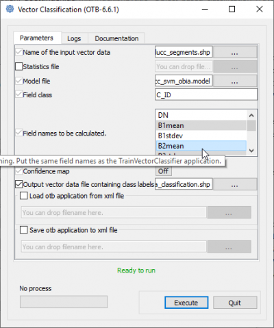
• In the search engine of mapla, type Vector and double click VectorClassifier.
• Name of the input vector data is lucc_segments.shp.
• Name of the input model file is lucc_svm_obia.model.
• Filed class is C_ID
• Mark in the list Field names to be calculated the same features as in the TrainVectorClassifier module (see above) using Ctrl + left-click).
• Specify the Output vector file. Execute