Supervised classification (Tutorial)
From AWF-Wiki
(Difference between revisions)
| Line 1: | Line 1: | ||
== Classification with Orfeo Toolbox == | == Classification with Orfeo Toolbox == | ||
=== Image statistics === | === Image statistics === | ||
| − | # Add the LandSat-8 imagery '' | + | # Add the LandSat-8 imagery ''Subset_S2A_MSIL2A_20170619T_B12_BOA.tif '' into a QGIS project. |
| − | # Calculate mean and standard error for each band of the | + | # Calculate mean and standard error for each band of the Sentinel-2 imagery. |
## Open {{mitem|text=Orfeo Toolbox --> Compute images second order statistics}} (see figure '''A'''). | ## Open {{mitem|text=Orfeo Toolbox --> Compute images second order statistics}} (see figure '''A'''). | ||
| − | ## Set '' | + | ## Set ''Subset_S2A_MSIL2A_20170619T_B12_BOA.tif'' as {{button|text=Input images}}. |
| − | ## Save the {{button|text=Output XML file}} as '' | + | ## Save the {{button|text=Output XML file}} as ''Subset_S2A_MSIL2A_20170619T_B12_BOA.tif.xml''. |
=== Train image classifier === | === Train image classifier === | ||
| − | # Add the training areas '' | + | # Add the training areas ''lab_9_training_input.shp'' into QGIS. It should be available in the course data. |
# Open {{mitem|text=Orfeo Toolbox --> TrainImageClassifier (libsvm)}} to use the Support Vector Machine SVM algorithm (see figure '''B'''). | # Open {{mitem|text=Orfeo Toolbox --> TrainImageClassifier (libsvm)}} to use the Support Vector Machine SVM algorithm (see figure '''B'''). | ||
| − | # Set '' | + | # Set ''Subset_S2A_MSIL2A_20170619T_B12_BOA.tif'' as {{button|text=Input image list}}. |
# Set ''training_manual_poly.shp'' as {{button|text=Input vector list}}. | # Set ''training_manual_poly.shp'' as {{button|text=Input vector list}}. | ||
| − | # Set '' | + | # Set ''Subset_S2A_MSIL2A_20170619T_B12_BOA.tif.xml'' as {{button|text=Input XML image statistics file}}. |
# Set {{button|text=Name of discrimination field}} to ''C_ID'' (C_ID refers to the column that contain the LUC classes code). | # Set {{button|text=Name of discrimination field}} to ''C_ID'' (C_ID refers to the column that contain the LUC classes code). | ||
# Save the {{button|text=Output confusion matrix}} as ''ConfusionMatrixSVM.csv''. | # Save the {{button|text=Output confusion matrix}} as ''ConfusionMatrixSVM.csv''. | ||
| Line 21: | Line 21: | ||
# Add the cloud mask ''cloud_shadow_mask.tif'' into QGIS. It should be available in the course data. | # Add the cloud mask ''cloud_shadow_mask.tif'' into QGIS. It should be available in the course data. | ||
# Open {{mitem|text=Orfeo Toolbox --> Image Classification}} (see figure '''C'''). | # Open {{mitem|text=Orfeo Toolbox --> Image Classification}} (see figure '''C'''). | ||
| − | # Set '' | + | # Set ''Subset_S2A_MSIL2A_20170619T_B12_BOA.tif'' as {{button|text=Input image}}. |
# Set ''cloud_shadow_mask.tif'' as {{button|text=Input mask}}. | # Set ''cloud_shadow_mask.tif'' as {{button|text=Input mask}}. | ||
# Set ''SVM.model'' as {{button|text=Model file}}. | # Set ''SVM.model'' as {{button|text=Model file}}. | ||
Revision as of 12:27, 11 December 2017
Contents |
Classification with Orfeo Toolbox
Image statistics
- Add the LandSat-8 imagery Subset_S2A_MSIL2A_20170619T_B12_BOA.tif into a QGIS project.
- Calculate mean and standard error for each band of the Sentinel-2 imagery.
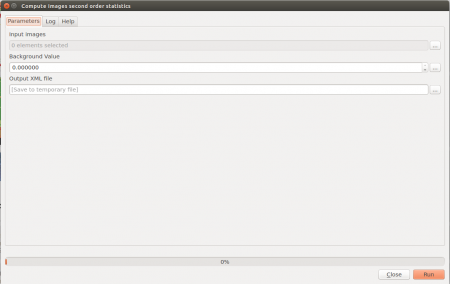
- Open Orfeo Toolbox --> Compute images second order statistics (see figure A).
- Set Subset_S2A_MSIL2A_20170619T_B12_BOA.tif as Input images.
- Save the Output XML file as Subset_S2A_MSIL2A_20170619T_B12_BOA.tif.xml.
Train image classifier
- Add the training areas lab_9_training_input.shp into QGIS. It should be available in the course data.
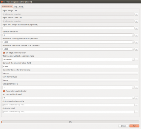
- Open Orfeo Toolbox --> TrainImageClassifier (libsvm) to use the Support Vector Machine SVM algorithm (see figure B).
- Set Subset_S2A_MSIL2A_20170619T_B12_BOA.tif as Input image list.
- Set training_manual_poly.shp as Input vector list.
- Set Subset_S2A_MSIL2A_20170619T_B12_BOA.tif.xml as Input XML image statistics file.
- Set Name of discrimination field to C_ID (C_ID refers to the column that contain the LUC classes code).
- Save the Output confusion matrix as ConfusionMatrixSVM.csv.
- Save the Output model as SVM.model.
- Calculation of accuracies :
Open ConfusionMatrixSVM.csv in LibreOffice or MS Excel and calculate overall, producer and consumer accuracies.
Classification
- Add the cloud mask cloud_shadow_mask.tif into QGIS. It should be available in the course data.
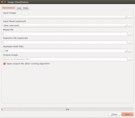
- Open Orfeo Toolbox --> Image Classification (see figure C).
- Set Subset_S2A_MSIL2A_20170619T_B12_BOA.tif as Input image.
- Set cloud_shadow_mask.tif as Input mask.
- Set SVM.model as Model file.
- Set SUB_LC81950242013188LGN00_MUL.tif.xml as Statistical file.
- Save the Output image as su_svm.tif.
- Evaluate classification results.
- Add the classification result su_svm.tif to QGIS.
- Right click su_svm.tif in the TOC and select Properties --> Style --> Style --> Load Style.
- Load classifcation.qml, which should be available in the course data.
- Open the Google Maps Layer under Web --> ObenLayers plugin --> Add Google Satellite layer and look for misclassification.
Compute a confusion matrix with independent reference data
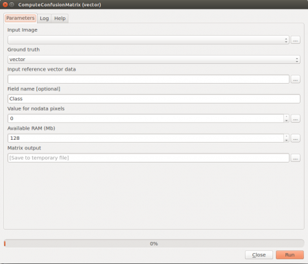
- Open Orfeo Toolbox --> ComputeConfusionMatrix (Vector) (see figure D).
- Set su_svm.tif as Input image.
- Set train_systematic_seg.shp as Input reference vector data.
- Set Field name to C_ID.


