|
|
| Line 1: |
Line 1: |
| − | {{construction}}
| |
| − | ''In this article, you will learn how to conduct a supervised image classification in [[QGIS]]''
| |
| − |
| |
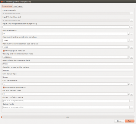
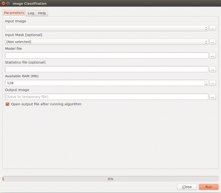
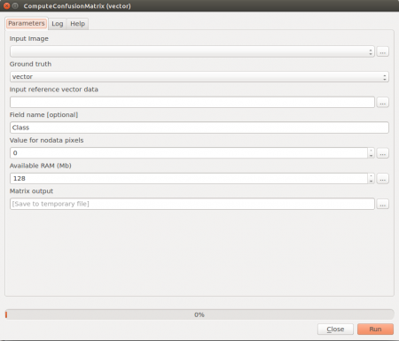
| | == Classification with Orfeo Toolbox == | | == Classification with Orfeo Toolbox == |
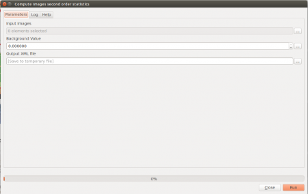
| | === Image statistics === | | === Image statistics === |
| Line 54: |
Line 51: |
| | | | |
| | | | |
| − |
| |
| − |
| |
| − | == Classification with Semi-Automatic Classification Plugin ==
| |
| − | === Plugin installation and testing ===
| |
| − | # Installing the plugin.
| |
| − | ## Click {{button|text=Manage and install plugins}}.
| |
| − | ## In the appearing menu, select {{button|text=Add more}}.
| |
| − | ## Browse for the {{button|text=Semi-Automatic Classification Plugin}} (it's most comfortable to use the search-field).
| |
| − | ## Click {{button|text=Install}}. If installation was successful, two additional windows should add to the [[QGIS GUI]] ({{button|text=Classification}} and {{button|text=ROI creation}}, see figure '''A''').
| |
| − | # Testing the plugin
| |
| − | ## For the plugin to work, you need to make sure that your installations of GRASS GIS, ORFEO Toolbox and SAGA GIS work correctly.
| |
| − | ## With the plugin installed, select {{mitem|text=Raster --> Semi Automatic Class Plugin}}.
| |
| − | ## In the appearing menu, select the {{button|text=Settings}} tab (figure '''B'''). Click {{button|text=Test Grass GIS}} and wait until the message {{button|text=Test OK}} appears. Do the same the Orfeo Toolbox, Saga and Qgis geoalgorithms.
| |
| − |
| |
| − | === Classification ===
| |
| − | # Add the raster map ''188_pca_indices.tif'' from the [[course data]] (see previous exercises).
| |
| − | # Also add the vector layer ''Training_manual_poly.shp''.
| |
| − |
| |
| − | ==== ROI digitalization ====
| |
| − | For better understanding of the workflow, try digitizing some
| |
| − | '''R'''egions '''O'''f '''I'''nterest yourself.
| |
| − | # First, you need to create a new shapefile to store the ROIs.
| |
| − | #* In the {{button|text=Input}} section of the {{button|text=ROI creation}} menu, click the {{button|text=New shapefile}} button. Just select the directory and file for the new shapefile and add it to the [[QGIS GUI|canvas]]. Click the {{button|text=Refresh list of shapefiles}} button and select your shapefile from the pulldown menu.
| |
| − | # In the {{button|text=ROI Definition}} section you can add define the attributes of each ROI. The {{button|text=Macroclass ID}}, which may be used to code sub-classes of the main classes (like e.g. ''Coniferous forest'' as a macroclass of ''Forest''), the {{button|text=Class ID}} and the name of the class in the {{button|text=Information}} column.
| |
| − | # As an example, enter {{typed|text=Urban area}} in the {{button|text=Information}} column and leave the ID's as they are.
| |
| − | # Looking at the {{button|text=ROI creation}} section, you see two options for generating the ROI:
| |
| − | #* By clicking {{button|text=+}}, you can select nondimensional points at the map. Simply place them in pixel clusters you have identified as belonging to the respective class. The regions will later be generated by ''region growing''.
| |
| − | #* A more precise way is to delineate ROI polygons using the {{button|text=Create a ROI polygon}} tool. You can re-draw the shape of a specific pixel cluster on the map and finish with a right-click.
| |
| − | # After having digitized a certain number of points or polygons for a ROI, click {{button|text=Save ROI}}. Wait until the computation is finished. You will then see the ROI being added to the {{button|text=ROI list}} in the {{button|text=Classification}} window.
| |
| − | # Repeat ROI generation for a few classes, like e.g.
| |
| − | #* Forest
| |
| − | #* Agricultural area
| |
| − | #* Water
| |
| − | #* Clouds
| |
| − | # After having added a few classe, select {{button|text=Minimum distance}} in the {{button|text=Classification algorithm}} section. Click {{button|text=+}} in the {{button|text=Classification preview}} section. By clicking somewhere on the map, a small preview for a section of the map will be generated.
| |
| − |
| |
| − | ==== Using predefined ROIs ====
| |
| − | Just adding a few classes will not generate a satisfying classification result. For a high quality classification, ROIs have to be very well defined, which requires a lot of time. For a supervised classification closer to real-life, you can use some predefined ROIs.
| |
| − | # Load the shapefile ''training_manual_poly.shp'' into the project and select it as training shapefile. You'll see how the ROI list is automatically updated.
| |
| − | # For {{button|text=Classification style}} click {{button|text=Select qml}} and browse for the file ''classification.qml'' from the [[course data]].
| |
| − | # In the {{button|text=Classification output}} section, check the {{button|text=Classificatin report}} and {{button|text=Calculate accuracy}} boxes.
| |
| − | # Click {{button|text=Perform classification}}. Enter name and path for the output map (e.g. ''ml_classification.tif'') and wait for the classification to finish (figure '''C'''). This may take a long time! Plan to do some different work (or just have lunch) while the algorithm is running.
| |
| − |
| |
| − | ==== Alternative algorithms and accuracy assessment ====
| |
| − | To get an impression of results depending on the alorithm selected, try the {{button|text=Maximum likelihood}} classifier as {{button|text=Classification algorithm}}.
| |
| − | In the {{button|text=Semi Automatic classification}} dialogue (figure '''D'''), select the {{button|text=Post processing}} tab to view the error matrix. If desired, it can be saved for future reference.
| |
| − |
| |
| − |
| |
| − |
| |
| − |
| |
| − | === Figures ===
| |
| − | {| class="wikitable" style="border:0pt"
| |
| − | |style="border:0pt"|[[Image:RemSens_Exercise08_02.png|thumb|450px|'''Figure A''': Dialogues of the ''Semi-Automatic Classification Plugin]]
| |
| − | |style="border:0pt"|[[Image:RemSens_Exercise08_01.png|thumb|450px|'''Figure B''': The ''Semi-Automatic Classification Plugin'' menu]]
| |
| − | |-
| |
| − | |style="border:0pt"|[[Image:RemSens_Exercise08_04.png|thumb|450px|'''Figure C''': The classified landcover map]]
| |
| − | |style="border:0pt"|[[Image:RemSens_Exercise08_05.png|thumb|450px|'''Figure D''': The ''Accuracy'' menu with error matrix]]
| |
| − | |}
| |
| | | | |
| | [[Category:Image classification]] | | [[Category:Image classification]] |


