Change detection
From AWF-Wiki
(Difference between revisions)
| Line 8: | Line 8: | ||
== Change detection techniques == | == Change detection techniques == | ||
=== Multi-temporal color composites === | === Multi-temporal color composites === | ||
| − | [[File:multi_temporal.png| | + | [[File:multi_temporal.png|250px]] |
==== Principal component analysis ==== | ==== Principal component analysis ==== | ||
# Add the raster layers of the years 1992 (''tm_920526_mul.tif''), 2005 (''etm_050623_mul.tif'') and 2010 (''etm_000515_mul.tif'') into a [[QGIS]] project. It should be available in the [[Course data|course data]]. | # Add the raster layers of the years 1992 (''tm_920526_mul.tif''), 2005 (''etm_050623_mul.tif'') and 2010 (''etm_000515_mul.tif'') into a [[QGIS]] project. It should be available in the [[Course data|course data]]. | ||
Revision as of 14:13, 1 February 2016
| sorry: |
This section is still under construction! This article was last modified on 02/1/2016. If you have comments please use the Discussion page or contribute to the article! |
Contents |
Prerequisites of multi-temporal image analysis
- Acquisition of remote sensing data by the same (or similar) sensor recorded using same spatial resolution, viewing geometry, spectral bands, time of day.
- Optical calibrationcorrecting uninteresting differences due to illumination, atmospheric conditions, topography, sensor calibration. DNs are converted to physical units (surface reflectance).
- Clear definitions and classification scheme
- Exact spatial coregistration
Change detection techniques
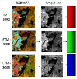
Multi-temporal color composites
Principal component analysis
- Add the raster layers of the years 1992 (tm_920526_mul.tif), 2005 (etm_050623_mul.tif) and 2010 (etm_000515_mul.tif) into a QGIS project. It should be available in the course data.
- Install PCA plugin under Plugins --> Manage and Install Plugins....
- Open PCA plugin pca.tif.
- Set tm_920526_mul.tif as Input Raster File.
- Set Number of output Principal Components to 1.
- Save the Output Raster File as pca1992_1.
- Repeat this procedure for the raster files of 2005 and 2010 and adapt the name of each Output Raster File.
- Merge the three output raster files with Toolbox --> GDAL/OGR --> [GDAL] Miscellaneous --> Merge and save Merged output as pca_merge.
Amplitude
- Add the raster layers of the years 1992 (tm_920526_mul.tif), 2005 (etm_050623_mul.tif) and 2010 (etm_000515_mul.tif) into a QGIS project. It should be available in the course data.
- Open Toolbox --> OTB --> Miscellaneous --> Band Math.
- Calculate the amplitude for each raster layer (1992, 2005, 2010) with the use of the bands 5-4-3.
- For the year 1992, set tm_920526_mul.tif as Input image list.
- Type sqrt(im1b4^2 + im1b5^2 + im1b3^2) as Expression.
- Save theOutput image as amplitude1992.
- Repeat this procedure for the raster files of 2005 and 2010 and adapt the name of each Output Raster File.
- Merge the three output images with Toolbox --> GDAL/OGR --> [GDAL] Miscellaneous --> Merge and save Merged output as amplitude_merge.
NDVI ratio
- Add the raster layers of the years 1992 (tm_920526_mul.tif) and 2005 (etm_050623_mul.tif) into a QGIS project. It should be available in the course data.
- Open Toolbox --> OTB --> Feature Extraction --> Radiometric indices.
- Set tm_920526_mul.tif as Input Image.
- Set Red Channel to 4 and NIR Channel to 5.
- Set Available Radiometric Indices to ndvi.
- Save the Output Image as ndvi1992.
- Repeat this procedure for the raster file of 2005 and adapt the name of the Output Image to ndvi_2005.
- Calculate the ratio of both raster images with the Band Math tool (Toolbox --> OTB --> Miscellaneous).
- Load ndvi_1992.tif and ndvi_2005 to the Input image list.
- Type im1b1/im2b1 as Expression.
- Save theOutput image as ndvi_ratio.
