Pair difference technique example
(→Example 1) |
(→Example 1) |
||
| Line 13: | Line 13: | ||
'''Table 1''' The population of all possible systematic samples of size <math>n=10</math> drawn from the example population. There are only 3 possibilities. PD-5 and 9 are the estimated error variances from the pair differences method with 5 non-overlapping and 9 overlapping pairs of sampled values. | '''Table 1''' The population of all possible systematic samples of size <math>n=10</math> drawn from the example population. There are only 3 possibilities. PD-5 and 9 are the estimated error variances from the pair differences method with 5 non-overlapping and 9 overlapping pairs of sampled values. | ||
| − | [[File:5.5.6.4-tab19.png| | + | [[File:5.5.6.4-tab19.png|left|400px|]] |
==References== | ==References== | ||
Revision as of 13:37, 23 December 2010
| Languages: |
English |
Example 1
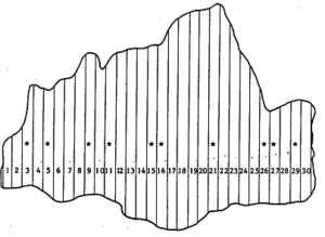
Systematic sampling from the example population in Figure 1 (Klein 2007[1]).

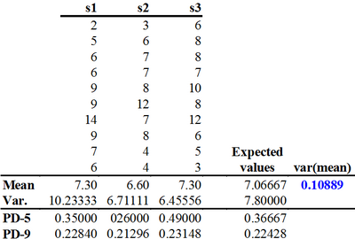
Taking a systematic sample of \(n=10\) elements, there are not many possibilities in our small example population. In fact, if the there shall be an equal distance between the elements in the list, this distance must be \(30/10=3\). Then, there are only three possible systematic samples having element 1, 2, or 3 as starting elements and then taking every third element. These three samples are listed and analyzed in Table 1.
Table 1 The population of all possible systematic samples of size \(n=10\) drawn from the example population. There are only 3 possibilities. PD-5 and 9 are the estimated error variances from the pair differences method with 5 non-overlapping and 9 overlapping pairs of sampled values.
References
- ↑ Kleinn, C. 2007. Lecture Notes for the Teaching Module Forest Inventory. Department of Forest Inventory and Remote Sensing. Faculty of Forest Science and Forest Ecology, Georg-August-Universität Göttingen. 164 S.
- ↑ de Vries, P.G., 1986. Sampling Theory for Forest Inventory. A Teach-Yourself Course. Springer. 399 p.
