Digitizing training and test areas

Revision as of 14:23, 4 June 2014

This article is part of the QGIS tutorial 2013/14.
During training phase we need to obtain the spectral reflectance, variability and range of digital images which are characteristic for categories that will be used in supervised classification approaches. This work step is very important for the results of a numerical classification. At first, we have to define the categories according to the objectives of the remote sensing study and the users's need. The training phase depends on previous knowledge acquired by previous field work or other sources of information like geometric high-resolution satellite images or aerial photos. Reference Information should be as close to the time of the image acquisition as possible. Image interpreters often use the technique of manual on-screen digitizing in vector mode to delineate and identify training areas. There are different opinions what is the best strategy to collect reference areas correctly. In general, digital image classifiers, accuracy and quality measures require statistical based sampling. Therefore we need to define a sampling- plot design in combination with an effective field survey. For accuracy assessment we need an additional independent data set of test areas. The sample size should be large enough to divide the reference data into training and test data.

Working steps

1. Generating sample points
   1. Load the raster map 188_pca_indices, which should be available in the course data.
   2. Open Vector --> Research tools --> regular points. If not selected by default, set the Input Boundary Layer to 188_pca_indices.
   3. Select the radio button Use this number of points and set the number to 50.
   4. Set Initial set from corner (LH side)
   5. Enter the file name and path by clicking Browse. You may use 188_pca_indices_points as a file name.
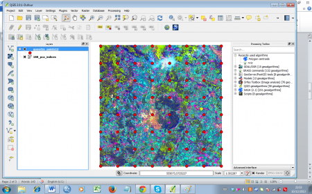
   6. Confirm with OK. Let the new layer be added to the TOC (figure A).
      • If the points are hard to recognize on the canvas, open the properties by double-clicking the layer in the TOC and adjusting size and color in the Style tab.
2. Buffering sample points
   1. Open Vector --> Geoprocessing tools --> Buffer. Select the generated points shapefile as input layer.
   2. Enter 200 (meter) as Buffer distance.
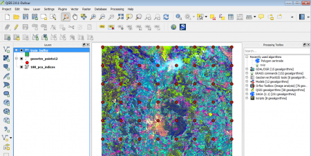
   3. Enter a file path and name, e.g. 188_pca_indices_buffer, confirm with OK and confirm the following dialogue to let the result be added to the project (figures B).
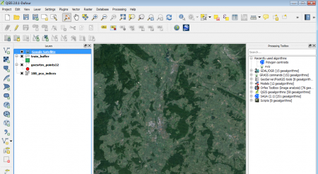
3. To get an overview of the terrain, you may add a google sattelite layer
   1. Select Plugins --> OpenLayers plugin --> Add Google Sattelite layer (figure C). Of course, you can also add a hybrid layer or try the layers from different providers.
      • If the Plugin doesn't exist in you QGIS installation, you'll first have to install it.
4. Create a new shapefile layer
   1. Select Layer --> New --> New Shapefile Layer.
      • As layer type, select Polygon. Click the Specify SRS button and select WGS 84/Pseudo Mercator (EPSG:3857).
      • To add an attibute:
        • For the attribute's name type (Class into the Name field of the New attribute section.
        • Select Whole number as data type.
        • Confirm with Add to attributes list.
      • Confirm with OK and enter the path and name (e.g. Training) in the following menu.
5. Digitizing areas
   1. Open the file digitizing_classes.pdf from the course data for a reference of landscape classes.
   2. Select the new shapefile in the TOC. Start the edit mode by clicking the Toggle editing button .
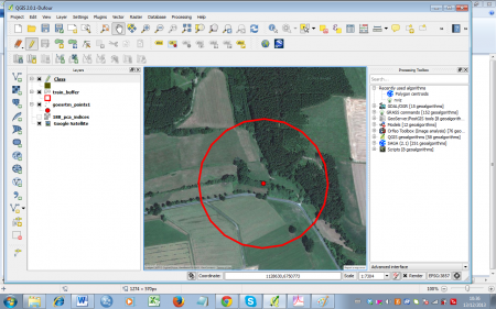
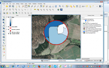
   3. Zoom in on a sample point (figure D). Click Add feature to start digitizing. Draw polygons according to the landscape classes. Simply click the desired point on the canvas to start. After selecting a second point, the third point will construct a triangle and each additional point will add another triangle to the geometry. Finish the geometry by right-clicking and entering the attributes in the appearing window (just use an increasing number for the ID). Take your time to get used to this way of digitizing -- you can always delete the last polygon by simply clicking Cancel in the attributes dialogue, or by selecting it and deleting with the Delete selected button. An example of a finished sample point can be seen in figure E.

Figures

Figure A: Map 188_pca_indices with sample points	Figure B: Buffered sample points
Figure C: Google satellite layer loaded via the Open layers plugin	Figure D: Zoom-in on buffered sample point with underlying Google satellite layer
Figure E: Example of a sample point after digitizing landscape classes