Supervised classification (Tutorial)
From AWF-Wiki
(Difference between revisions)
| (85 intermediate revisions by 2 users not shown) | |||
| Line 1: | Line 1: | ||
| − | + | =Per pixel classification with QGIS and OTB processing plugin= | |
| − | '' | + | In '''OTB Version 7.0.0''' the requirements for the input training vector data are very restrictive because of some bugs. |
| + | ** File format needs to be Shapefile (GPKG does not work). | ||
| + | ** The column containing the class label needs to integer (whole number). '''Data type Integer 64bit does not work!''' | ||
| + | ** Any other columns with other data types (real or text (string) with umlauts or blank are not correctly imported which leads to failure of the modul TrainImagesClassifier. | ||
| + | A work around is to make a copy of your training data and delete all other columns than the class label column | ||
| − | + | All these issues have been fixed in '''OTB Version 7.1.0'''! | |
| − | + | ||
| − | + | ||
| − | + | ||
| − | + | ||
| − | + | ||
| − | + | ||
| − | == | + | ==Training phase== |
| − | + | * In the search engine of Processing Toolbox, type {{typed|text=TrainImages}} and open '''TrainImagesClassifer'''. | |
| − | + | * In the {{button|text=Input Image List}} select a (or optional: several) multispectral images: '''mosaic_S2A_MSIL2A_20200521T102031_N0214_R065_T32UNC_UNB_UPC.tif'''. | |
| − | + | * In the {{button|text=Input Vector Data List}} choose a vector polygon file with training areas: '''lucc_training_2020-05-21.shp'''. | |
| − | + | * In the {{button|text=Validation Vector Data List}} and choose a vector polygon file with an independent sample of validation areas: leave empty. | |
| − | + | * Training and validation sample ratio: {{typed|text=0.25}}. This is a 4-fold cross-validation with split 0.75 per cent for training and 0.25 per cent for testing. | |
| − | + | * Type {{typed|text=Code}} in the {{button|text=Field Name}} text field. | |
| − | + | * Choose Support Vector Machine Classifer {{button|text=libsvm}} from the drop down list. | |
| − | + | * SVM Model Type is {{button|text=csvc}} | |
| − | + | * User defined input centroids: Type any character, no need for a filename. This field is required and but ignored (a bug in the OTB plugin!) | |
| + | * The SVM Kernel Type is {{button|text=Linear}}. | ||
| + | * Switch checkbox {{button|text=Parameters optimization}} '''off'''. The optimization results in a higher accuracy but takes much time (> 1 hour computation). | ||
| + | * In the {{button|text=Output model}} specify an model file: e.g. '''svm.model''' | ||
| + | * Define an output file for {{button|text=Output confusion matrix or contingency table}} (e.g.'''svm_matrix.csv'''). | ||
| + | * Click {{button|text=Run}}. | ||
| + | * Click on the {{button|text=Log}} tab and inspect the '''model quality''' measures: Precision, Recall, F-score and Kappa index. | ||
| + | [[File:qgis_otb_trainimages.png|400px]] | ||
| − | + | ==Classification phase== | |
| − | + | * In the search engine of Processing Toolbox, type {{typed|text=ImageClassifier}} and double click '''ImageClassifier'''. | |
| − | + | * Set ''mosaic_S2A_MSIL2A_20200521T102031_N0214_R065_T32UNC_UNB_UPC.tif'' as {{button|text=Input image}}. | |
| − | + | * Set {{button|text=Input _mask}} to blank (top of drop-down list). | |
| − | + | * Set '''lucc_svm.model''' as {{button|text=Model file}}. | |
| − | + | * Set the number of classes in your model: this is the number of unique classes in your training file. | |
| − | + | * Set {{button|text=Output pixel type}} to '''uint16''' | |
| − | + | * Save the {{button|text=Output image}} as '''svm_classification.tif'''. | |
| − | + | * Uncheck Confidence map: ''Open output file after running algorithm''. | |
| − | + | * Uncheck Probability map: ''Open output file after running algorithm''. | |
| − | + | * Add ''svm_classification.tif'' to QGIS canvas. | |
| − | + | * Find the prepared style file '''rast_classifcation.qml''' in the Tutorial data of Workshop 05. | |
| − | + | * Right click ''svm_classification.tif'' in the [[TOC]] and select {{mitem|text=Properties --> Symbology --> Style --> Load Style}}. | |
| + | * Select the style file '''svm_classification.tif'''. {{button|text=OK}}. | ||
| + | [[File:qgis_otb_imageclassifier.png|400px]] | ||
| − | === | + | ==Postprocessing== |
| − | + | This application uses a majority filter with a circular structure element. | |
| − | + | * In the search engine of Processing Toolbox, type {{typed|text=regularization}} and double click '''ClassificationMapRegularization'''. | |
| − | + | * Define {{button|text=Input classification image}} as an classification output raster. | |
| − | + | * Set {{button|text=Structuring element radius}} to {{typed|text=2}} pixels. | |
| + | * Set {{button|text=Output pixel type}} to {{button|text=uint16}}. | ||
| + | * Save the {{button|text=Output regularizd image}} as '''svm_classification_majority.tif'''. | ||
| + | * Click {{button|text=Run}}. | ||
| + | [[File:qgis_otb_majority.png|400px]] | ||
| + | =Per pixel classification with OTB standalone= | ||
| + | ==Training phase== | ||
| + | * Type into the search box of the Windows taskbar: {{typed|text=mapla.bat}}. Click on mapla.bat to open Monteverdi Application Launcher. | ||
| + | * In the search engine of mapla, type {{typed|text=TrainImages}} and double click '''TrainImagesClassifer'''. | ||
| + | * In the {{button|text=Input Image List}} click on {{button|text=+}} and select a (or optional: several) multispectral images: '''Subset_S2A_MSIL2A_20170619T_MUL.tif '''. | ||
| + | * In the {{button|text=Input Vector Data List}} choose a vector polygon file with training areas: '''lucc_training_input.shp'''. | ||
| + | * Activate the checkbox {{button|text=Validation Vector Data List}} and choose a vector polygon file with an independent sample of validation areas: '''lucc_validation.shp''' | ||
| + | * In the {{button|text=Output model}} specify an output model file: e.g. '''lucc_svm.model''' | ||
| + | * Activate the checkbox and save the {{button|text=Output confusion matrix or contingency table}} as '''lucc_svm_confusion.csv'''. | ||
| + | * In the {{button|text=Bound sample number by minimum}} field type {{typed|text=1}}. | ||
| + | * Set the {{button|text=training and validation sample ratio}} to {{typed|text=0 }}. (0 = all training data). | ||
| + | * Mark ''C_ID'' in the {{button|text=Field containing the class integer label}} (C_ID refers to the column that contains the LUC code in the training and validation vector file). | ||
| + | * Choose {{button|text=LibSVM classifier}} from the drop down list as Classifier to use for the training. | ||
| + | * The SVM Kernel Type is {{button|text=Linear}}. | ||
| + | * The SVM Model Type is {{button|text=C support vector classification}}. | ||
| + | * Switch the Parameters optimization to {{button|text=on}}. | ||
| + | * Check user defined seed and enter an integer value. | ||
| + | * Click on {{button|text=Execute}}. | ||
| + | * Click on the {{button|text=Log}} tab and inspect the quality measures: Precision, Recall, F-score and Kappa index. | ||
| + | [[File:otb_trainimages.png|500px]] | ||
| + | ==Classification phase== | ||
| + | * In the search engine of mapla, type {{typed|text=ImageClassifier}} and double click '''ClassifcationMapRegularization''' | ||
| + | * Set ''Subset_S2A_MSIL2A_20170619T_MUL.tif'' as {{button|text=Input image}}. | ||
| + | * Set '''SVM.model''' as {{button|text=Model file}}. | ||
| + | * Save the {{button|text=Output image}} as '''svm_classification.tif'''. | ||
| + | [[File:otb_imageclassifier.png|500px]] | ||
| + | * Evaluate classification results: | ||
| + | * Add ''svm_classification.tif'' to QGIS canvas. | ||
| + | * Download the style file '''classifcation.qml''' from Stud.IP. | ||
| + | * Right click ''svm_classification.tif'' in the [[TOC]] and select {{mitem|text=Properties --> Style --> Style --> Load Style}}. | ||
| + | * Select the style file '''\lucc\classification.qml'''. {{button|text=OK}}. | ||
| + | * Open the text file '''lucc_svm_confusion.csv''' with LibreOffice Calc or MS Excel and calculate overall, user, producer accuracy and kappa index. | ||
| − | + | ==Postprocessing== | |
| − | == | + | This application uses a majority with a circular structure element. |
| − | + | * In the search engine of mapla, type, {{typed|text=regular}} and double click '''ClassifcationMapRegularization'''. | |
| − | + | * Define {{button|text=Input classification image}} as ans classification output raster. | |
| − | + | * Save the {{button|text=Output regularizd image}} as '''svm_classification_majority.tif'''. | |
| − | + | * Set {{button|text=Structuring element radius}} to {{typed|text=3}} pixels. | |
| − | + | * Set {{button|text=Output pixel type}} to {{button|text=uint8}}. | |
| − | + | * Click {{button|text=Execute}}. | |
| − | + | [[File:otb_majority.png|400px]] | |
| − | + | ||
| − | + | ||
| − | + | ||
| − | + | ||
| − | + | ||
| − | + | ||
| − | + | ||
| − | + | ||
| − | + | ||
| − | + | ||
| − | + | ||
| − | + | ||
| − | + | ||
| − | + | ||
| − | + | ||
| − | + | ||
| − | + | ||
| − | + | ||
| − | + | ||
| − | + | ||
| − | + | ||
| − | + | ||
| − | + | ||
| − | + | ||
| − | + | ||
| − | + | ||
| − | + | ||
| − | + | ||
| − | + | ||
| − | + | ||
| − | + | ||
| − | + | ||
| − | + | ||
| − | + | ||
| − | + | ||
| − | + | ||
| − | + | ||
| − | + | ||
| − | + | ||
| − | + | ||
| − | + | ||
| − | + | ||
| − | + | ||
| − | + | ||
| − | + | ||
| − | + | ||
| − | + | ||
| − | + | ||
| − | + | ||
| − | + | ||
| − | + | ||
| − | + | ||
| − | + | ||
| − | + | ||
| − | + | ||
| − | + | ||
| − | + | ||
| − | + | ||
| − | + | ||
| − | + | ||
| − | + | ||
| − | + | ||
Latest revision as of 14:12, 1 December 2020
Contents |
[edit] Per pixel classification with QGIS and OTB processing plugin
In OTB Version 7.0.0 the requirements for the input training vector data are very restrictive because of some bugs.
- File format needs to be Shapefile (GPKG does not work).
- The column containing the class label needs to integer (whole number). Data type Integer 64bit does not work!
- Any other columns with other data types (real or text (string) with umlauts or blank are not correctly imported which leads to failure of the modul TrainImagesClassifier.
A work around is to make a copy of your training data and delete all other columns than the class label column
All these issues have been fixed in OTB Version 7.1.0!
[edit] Training phase
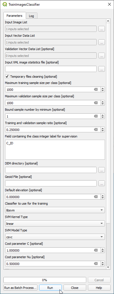
- In the search engine of Processing Toolbox, type TrainImages and open TrainImagesClassifer.
- In the Input Image List select a (or optional: several) multispectral images: mosaic_S2A_MSIL2A_20200521T102031_N0214_R065_T32UNC_UNB_UPC.tif.
- In the Input Vector Data List choose a vector polygon file with training areas: lucc_training_2020-05-21.shp.
- In the Validation Vector Data List and choose a vector polygon file with an independent sample of validation areas: leave empty.
- Training and validation sample ratio: 0.25. This is a 4-fold cross-validation with split 0.75 per cent for training and 0.25 per cent for testing.
- Type Code in the Field Name text field.
- Choose Support Vector Machine Classifer libsvm from the drop down list.
- SVM Model Type is csvc
- User defined input centroids: Type any character, no need for a filename. This field is required and but ignored (a bug in the OTB plugin!)
- The SVM Kernel Type is Linear.
- Switch checkbox Parameters optimization off. The optimization results in a higher accuracy but takes much time (> 1 hour computation).
- In the Output model specify an model file: e.g. svm.model
- Define an output file for Output confusion matrix or contingency table (e.g.svm_matrix.csv).
- Click Run.
- Click on the Log tab and inspect the model quality measures: Precision, Recall, F-score and Kappa index.
[edit] Classification phase
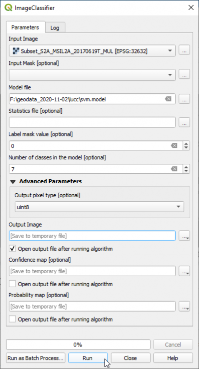
- In the search engine of Processing Toolbox, type ImageClassifier and double click ImageClassifier.
- Set mosaic_S2A_MSIL2A_20200521T102031_N0214_R065_T32UNC_UNB_UPC.tif as Input image.
- Set Input _mask to blank (top of drop-down list).
- Set lucc_svm.model as Model file.
- Set the number of classes in your model: this is the number of unique classes in your training file.
- Set Output pixel type to uint16
- Save the Output image as svm_classification.tif.
- Uncheck Confidence map: Open output file after running algorithm.
- Uncheck Probability map: Open output file after running algorithm.
- Add svm_classification.tif to QGIS canvas.
- Find the prepared style file rast_classifcation.qml in the Tutorial data of Workshop 05.
- Right click svm_classification.tif in the TOC and select Properties --> Symbology --> Style --> Load Style.
- Select the style file svm_classification.tif. OK.
[edit] Postprocessing
This application uses a majority filter with a circular structure element.
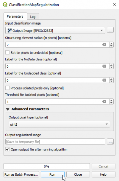
- In the search engine of Processing Toolbox, type regularization and double click ClassificationMapRegularization.
- Define Input classification image as an classification output raster.
- Set Structuring element radius to 2 pixels.
- Set Output pixel type to uint16.
- Save the Output regularizd image as svm_classification_majority.tif.
- Click Run.
[edit] Per pixel classification with OTB standalone
[edit] Training phase
- Type into the search box of the Windows taskbar: mapla.bat. Click on mapla.bat to open Monteverdi Application Launcher.
- In the search engine of mapla, type TrainImages and double click TrainImagesClassifer.
- In the Input Image List click on + and select a (or optional: several) multispectral images: Subset_S2A_MSIL2A_20170619T_MUL.tif .
- In the Input Vector Data List choose a vector polygon file with training areas: lucc_training_input.shp.
- Activate the checkbox Validation Vector Data List and choose a vector polygon file with an independent sample of validation areas: lucc_validation.shp
- In the Output model specify an output model file: e.g. lucc_svm.model
- Activate the checkbox and save the Output confusion matrix or contingency table as lucc_svm_confusion.csv.
- In the Bound sample number by minimum field type 1.
- Set the training and validation sample ratio to 0. (0 = all training data).
- Mark C_ID in the Field containing the class integer label (C_ID refers to the column that contains the LUC code in the training and validation vector file).
- Choose LibSVM classifier from the drop down list as Classifier to use for the training.
- The SVM Kernel Type is Linear.
- The SVM Model Type is C support vector classification.
- Switch the Parameters optimization to on.
- Check user defined seed and enter an integer value.
- Click on Execute.
- Click on the Log tab and inspect the quality measures: Precision, Recall, F-score and Kappa index.
[edit] Classification phase
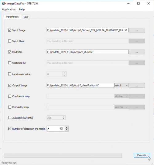
- In the search engine of mapla, type ImageClassifier and double click ClassifcationMapRegularization
- Set Subset_S2A_MSIL2A_20170619T_MUL.tif as Input image.
- Set SVM.model as Model file.
- Save the Output image as svm_classification.tif.
- Evaluate classification results:
- Add svm_classification.tif to QGIS canvas.
- Download the style file classifcation.qml from Stud.IP.
- Right click svm_classification.tif in the TOC and select Properties --> Style --> Style --> Load Style.
- Select the style file \lucc\classification.qml. OK.
- Open the text file lucc_svm_confusion.csv with LibreOffice Calc or MS Excel and calculate overall, user, producer accuracy and kappa index.
[edit] Postprocessing
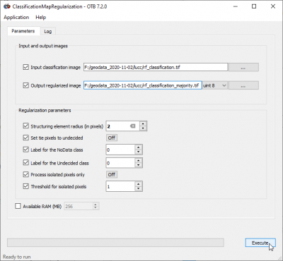
This application uses a majority with a circular structure element.
- In the search engine of mapla, type, regular and double click ClassifcationMapRegularization.
- Define Input classification image as ans classification output raster.
- Save the Output regularizd image as svm_classification_majority.tif.
- Set Structuring element radius to 3 pixels.
- Set Output pixel type to uint8.
- Click Execute.

