Change detection
(→Time series viewer) |
(→Raster algebra: Ratio) |
||
| (3 intermediate revisions by one user not shown) | |||
| Line 82: | Line 82: | ||
Mask Layer: '''mask_FTY_2015_Coniferous_poly.gpkg''' | Mask Layer: '''mask_FTY_2015_Coniferous_poly.gpkg''' | ||
* Mark the masked difference NDVI image right click {{mitem|text=Properties --> i Information}} [[Image:QGIS_2.0_metadata_info.png|100px]]. In the "properties" window scroll down and report mean STATISTICS_MEAN and standard deviation STATISTICS_STDDEV. | * Mark the masked difference NDVI image right click {{mitem|text=Properties --> i Information}} [[Image:QGIS_2.0_metadata_info.png|100px]]. In the "properties" window scroll down and report mean STATISTICS_MEAN and standard deviation STATISTICS_STDDEV. | ||
| − | * Find threshold values for forest change areas: Calculate | + | * Find threshold values for forest change areas: Calculate (e.g., with MS Calculator app) |
threshold 1 = mean - 2 * stddev and | threshold 1 = mean - 2 * stddev and | ||
threshold 2 = mean + 2 * stddev. | threshold 2 = mean + 2 * stddev. | ||
| − | * {{mitem|text=Layer Properties --> Histogram}} | + | * {{mitem|text=Layer Properties --> Histogram}} Compute a difference histogram. |
* {{mitem|text=Layer Properties --> Symbology}}. Change Render type to {{button|text=Singleband Pseudocolor}} | * {{mitem|text=Layer Properties --> Symbology}}. Change Render type to {{button|text=Singleband Pseudocolor}} | ||
| − | * | + | * Choose '''Min / max''' in the Min / Max value Settings. |
* Choose Accuracy: {{button|text=Actual(Slower)}} and click {{button|text=Apply}}. | * Choose Accuracy: {{button|text=Actual(Slower)}} and click {{button|text=Apply}}. | ||
* Choose Interpolation: {{button|text=Discrete}}. | * Choose Interpolation: {{button|text=Discrete}}. | ||
| − | * Select a color | + | * Select a color ramp. In the Drop Down Menu choose {{button|text=Spectral}} and {{button|text=Invert Color Ramp}}. |
| − | * | + | * For Classes choose {{typed|text=3}}. |
* Adjust the thresholds according to your results: Type e.g, | * Adjust the thresholds according to your results: Type e.g, | ||
for Value <= :first line: {{typed|text=-0.23}} (threshold 1) | for Value <= :first line: {{typed|text=-0.23}} (threshold 1) | ||
| Line 102: | Line 102: | ||
=== Raster algebra: Ratio === | === Raster algebra: Ratio === | ||
Calculate the ratio of NDVI images 2017 ('''ndvi_date1''') and 2018 ('''ndvi_date2''') with the {{mitem|text=Raster --> Raster Calculator}}. | Calculate the ratio of NDVI images 2017 ('''ndvi_date1''') and 2018 ('''ndvi_date2''') with the {{mitem|text=Raster --> Raster Calculator}}. | ||
| − | + | * Choose ''ndvi_2018@1'' ('''ndvi_date2''') from the {{button|text=Raster bands}} by double clicking on the raster name. | |
| − | + | * Choose the division operator from the {{button|text=Operators}} by clicking on {{button|text= / }}. | |
| − | + | * Choose ''ndvi_2017@1.tif'' ('''ndvi_date1''') from the {{button|text=Raster bands}} by double clicking on the raster name. | |
| − | + | * Save the {{button|text=Output layer}} as ''ndvi_ratio'' and press {{button|text=OK}}. | |
| + | * Mask the ratio image with a coniferous forest mask: {{mitem|text=Raster --> Extraction --> Clip raster by mask layer}} | ||
| + | Mask Layer: '''mask_FTY_2015_Coniferous_poly.gpkg'''. | ||
=== Raster algebra: Change vector analysis === | === Raster algebra: Change vector analysis === | ||
| Line 153: | Line 155: | ||
=== Principal component analysis === | === Principal component analysis === | ||
| − | * Stack three | + | * Stack three Sentinel-2 multispectral images from three different years 2018,2019,2020 with {{mitem|text=Toolbox --> GDAL/OGR --> [GDAL] Miscellaneous --> Merge}}. See also [[Create stack]]. |
| − | * Perform a [[Principal component analysis]] on the stacked | + | * Perform a [[Principal component analysis]] on the stacked 27 bands of the multitemporal Sentinel-2 image stack. Enter 5 as number of components and visualize them as color comoposite. |
[[category:QGIS Tutorial]] | [[category:QGIS Tutorial]] | ||
Latest revision as of 15:33, 18 January 2021
Contents |
[edit] Pre-requisites of spatio-temporal image analysis
Correct the pixel intensities as much as possible for uninteresting differences:
- Sensor calibration
- Exact spatial co-registration of images (especially pixel-by-pixel comparision)
- Cloud and cloud shadow masking
- Haze reduction
- Atmospheric correction
- Topographic illumination correction (mountains)
- Clear definitions and classification scheme
[edit] Visualization of bi-temporal Sentinel-2 images (pre-event and post-event)
- Add subsets of Sentinel-2 multispectral scenes of August 2017 (subset_SA2_2017-08-15_MUL.tif) before the storm events, and May 2018 (subset_SA2_2018-05-07_MUL.tif) after storm events into the QGIS TOC.
- Create color composites RGB=9-7-3 Changing Raster Layer Style of a multiband file.
- Load the map (EMSR266_14BADGRUND_01DELINEATION_MAP_v1_300dpi.tif) showing the storm situation near Bad Grund in the Harz mountains after the winter storm Friederike. Change the Layer Style setting to RGB=1-2-3.
The map was produced by the European Copernicus EMS Rapid Mapping activity with the aim to provide an overview of the forest damages based on visual interpretation of very high resolution Pleiades satellite images (pre- and post-event).
- Load the shapefile EMSR266_14BADGRUND_DEL_v1_observed_event_a_EPSG32632.shp which contains delineated areas with loss of tree cover on top of the EMS map Bad Grund.
[edit] Globe plugin
- Currently the Globe plugin is not availabe for QGIS 3 and works only for QGIS 2. If it is already installed it just needs to be activated.
Plugins --> Manage and Install Plugins --> Installed. Click the checkbox or doubleclick the name Globe to activate the plugin.
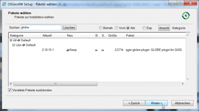
- If the Globe plugin is not installed it may be be installed via the QSGeo4W setup as shown below.
- Plugins --> Globe --> Launch Globe. The Globe windows opens side by side to the map canvas.
- In the Globe viewer click on Globe settings
 . Switch off the atmosphere rendering by unchecking the box Sky. OK.
- Adjust the size of the Globe viewer to the same size as the map canvas.
- In the map canvas zoom in to a region of interest. Adjust the local histogram stretch for all layers in the TOC clicking
 (Raster Tools).
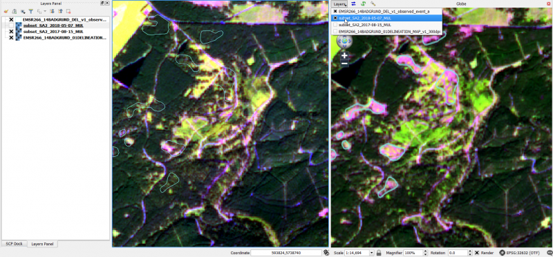
- In the Globe Viewer click on Layerand check the layers that you would like to see on top of the Globe Viewer.
- Click first on Reload layer
 and then Synchronize extent
  . The extents of the canvas (left: 2017) and the Globe viewer (right: 2018) are synchronized as shown below.
[edit] MapSwipe Tool plugin
This plugin is a map tool for swipe active layer, for example, you can see the difference with other layers below. The active layer, or group, will appear above all others.
- Select Plugins --> MapSwipe Tool or click
 . If the Plugin doesn't exist you'll first have to install it. Check Plugins --> Manage and Install plugins.. --> Settings Show also experimental plugins.
- Mark a layer below the top layer in the TOC and hold left click to blend to and compare two layers.
- You can also use Google Satellite as active layer!
[edit] Temporal/Spectral Profile plugin
This plugin is for interactive plotting of temporal or spectral information stored in multi-band rasters.
After installation and activation the plugin can be accessed either from main menu Plugins --> Profile Tool --> Temporal/Spectral Profile) or from an icon ![]() on the taskbar.
on the taskbar.
[edit] Plot different dates of multispectral images
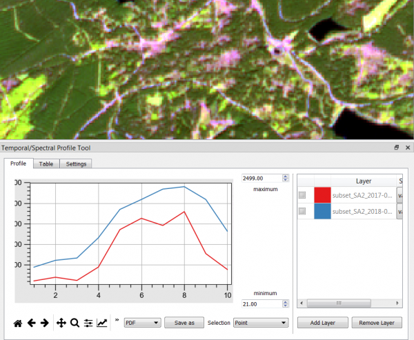
- Load 2 multispectral Sentinel-2 files from different dates into the QGIS legend (TOC).
- Mark the layer name of first date in the TOC.
- Click
 to open the Temporal/Spectral Profile Tool.
- Mark the layer name of second date in the TOC and click Add Layer
- Click on a location in the canvas.
[edit] Plot times series of stacked NDVI images
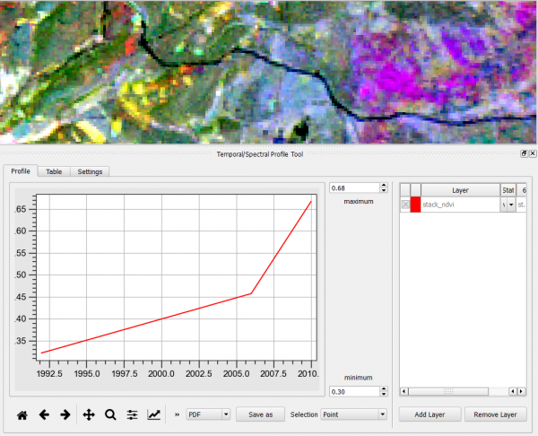
- Load a temporal stack of NDVI images of different dates into the TOC.
- Mark the layer name in the TOC
- Click
 to open the Temporal/Spectral Profile Tool.
- Select as X-axis steps Settings --> From string.
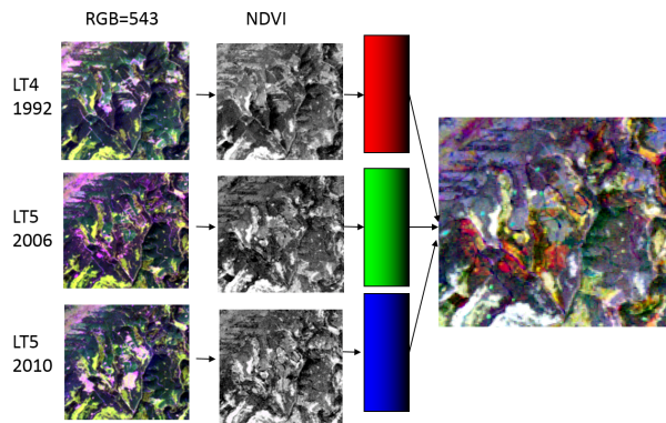
- Type in the text field the years or dates of the NDVI images (e.g. 1992;2006;2010)
- Click on a location in the canvas.
[edit] Change detection techniques
[edit] Bitemporal
[edit] Post-classification Comparison
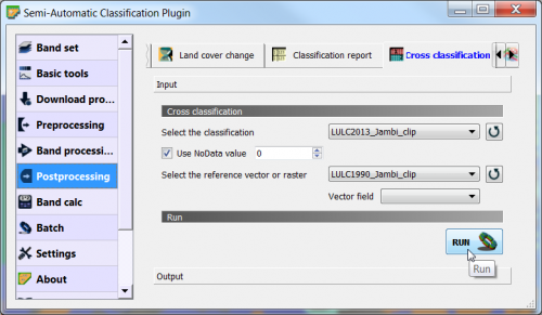
This is an indirect change detection method: First two co-registered satellite images are independently classified to yield thematic maps. Then, discrete class labels of two thematic raster layers are compared to determine changes using cross-tabulation in which all transitions are presented. Use the Semi Automatic Classification plugin: SCP --> Postprocessing --> Cross classification
[edit] Raster algebra: Difference
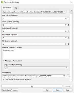
- In the search engine of the Processing Toolbox Toolbox (or mapla.bat in the standalone OTB), type Radiometric and select Radiometric Indices under Feature Extraction of the Orfeo Toolbox.
- Select the Sentinel-2 SA2_2017-08-23.tif file as input layer (image_date1).
- Assign the spectral bands to the right band number as shown below.
- Type: Vegetation:NDVI in the Available Radiometric Indices Window to calculate the Normalized Difference Vegetation Index.
- Enter name and path for an output file.
- Click on Run.
- Calculate also the NDVI of the Sentinel-2 image SA2_2018-07-19.tif (image_date2).
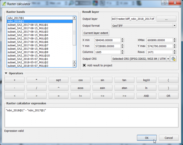
- Calculate the difference between the NDVI 2018 and NDVI 2017 (ndvi_date2 - ndvi_date1) using the Raster Calculator.
- Click Raster --> Raster calculator.
- A difference NDVI is calculated by the expression as shown below.
- Define path and file name of the output layer. OK.
- Mask the difference image with a coniferous forest mask:
Raster --> Extraction --> Clip raster by mask layer Mask Layer: mask_FTY_2015_Coniferous_poly.gpkg
- Mark the masked difference NDVI image right click Properties --> i Information
 . In the "properties" window scroll down and report mean STATISTICS_MEAN and standard deviation STATISTICS_STDDEV.
- Find threshold values for forest change areas: Calculate (e.g., with MS Calculator app)
threshold 1 = mean - 2 * stddev and threshold 2 = mean + 2 * stddev.
- Layer Properties --> Histogram Compute a difference histogram.
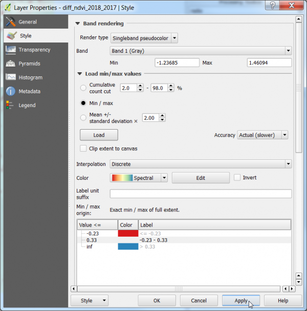
- Layer Properties --> Symbology. Change Render type to Singleband Pseudocolor
- Choose Min / max in the Min / Max value Settings.
- Choose Accuracy: Actual(Slower) and click Apply.
- Choose Interpolation: Discrete.
- Select a color ramp. In the Drop Down Menu choose Spectral and Invert Color Ramp.
- For Classes choose 3.
- Adjust the thresholds according to your results: Type e.g,
for Value <= :first line: -0.23 (threshold 1) second line +0.33 (threshold 2)
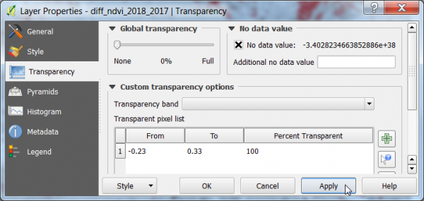
- Layer Properties --> Transparency. Click
 to add a new line in the pixel transparency list. Type values From: -0.23 and To: 0.33. OK. The specified range of the difference raster is now transparent and can be overlaid on top of Google Satellite and Sentinel composites.
[edit] Raster algebra: Ratio
Calculate the ratio of NDVI images 2017 (ndvi_date1) and 2018 (ndvi_date2) with the Raster --> Raster Calculator.
- Choose ndvi_2018@1 (ndvi_date2) from the Raster bands by double clicking on the raster name.
- Choose the division operator from the Operators by clicking on /.
- Choose ndvi_2017@1.tif (ndvi_date1) from the Raster bands by double clicking on the raster name.
- Save the Output layer as ndvi_ratio and press OK.
- Mask the ratio image with a coniferous forest mask: Raster --> Extraction --> Clip raster by mask layer
Mask Layer: mask_FTY_2015_Coniferous_poly.gpkg.
[edit] Raster algebra: Change vector analysis
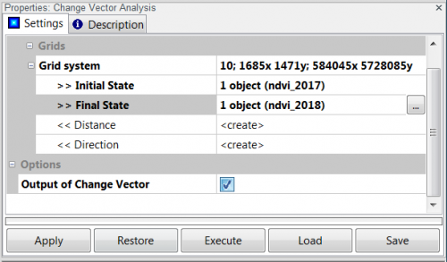
- Type into the Windows search field saga and click SAGA GIS.
- Load files: In the Manager windows choose the Data tab. Drag and drop the files ndvi_2017.tif and ndvi_2018.tif from Windows file explorer into the Data tab.
- Click Tools --> Grid --> Analysis --> Change Vector Analysis.
- Specify Grid system.
- Input features are supplied as ndvi_2017.tif for Inital State and ndvi_2018.tif for Final State. In case two or more grids are used as features the same layer order has to be defined in both lists. Distance is measured as Euclidean distance in features space. When analyzing two features direction is calculated as angle (radians) by default. Otherwise direction is coded as the quadrant it points to in terms of feature space.
- Check Output of change vector.
- Click Execute.
- Click Geoprocessing --> File --> Grid --> Export --> Export Geotiff.
- Specify Grid system.
- As Grid choose Change vector 1.
- Choose name and path for the output file.
- Click OK.
- Open the file in QGIS and choose a color table in Layer properties --> Symbology --> Band rendering --> Singleband pseudocolor
[edit] Change classification
The resulting layers of raster algebra are classified according to specific change types. In case we are only interested in changes of one land cover type (e.g. coniferous forest) we use a clipped difference image with mask layer mask_FTY_2015_Coniferous_poly.gpkg extracted from class 2 = coniferous forest of the pan-european Copernicus Land Cover product Forest Type 2015.
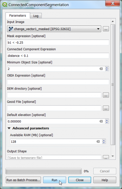
- In the search engine of the Processing Toolbox type connected and select ConnectedComponentSegmentation under Segmentation of the Orfeo Toolbox.
- Under the Parameter tab, select the raster file diff_ndvi_2018_2017_masked.tif as input layer.
- Type the mask expression b1 < -0.25 (or try other lower thresholds).
- Type the connected component expression distance < 0.1.
- Save a permanent output file with "gpkg” extension).
- Click on Run to execute the algorithm.
[edit] Bi-temporal color composite
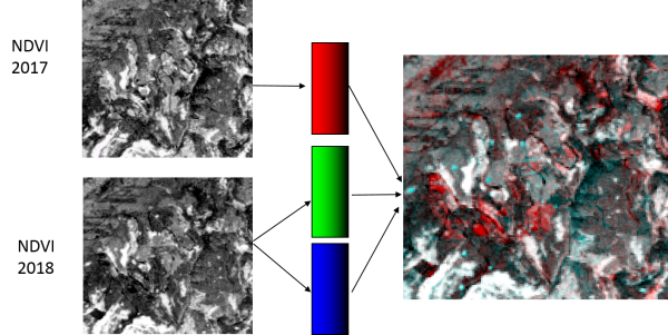
- Stack two or three ndvi raster files from three different dates with Toolbox --> GDAL--> RASTER --> Miscellaneous --> Build Virtual Raster. See also Create stack.
- Layer Properties --> Symbology. Assign two ndvi images to RGB colors.
- Red, cyan: high value in one date and low in the others. Change from one date to the other.
- Gray levels: indicate features are unchanged.
[edit] Multi-temporal
[edit] Multi-temporal color composite
- Stack three ndvi raster files from three different dates with Toolbox --> GDAL/OGR --> [GDAL] Miscellaneous --> Merge. See also Create stack.
- Layer Properties --> Style. Assign the three ndvi images to RGB colors.
- Red, green, blue: high value in one date and low in the others. Change from one date to the other and invariant afterwards
- Gray levels: indicate features are stable in all dates.
- Yellow (R+G), cyan (G+B), or magenta (R+B): high values in two dates and low in the other. Change from two dates to the third one.
Use the EO Time Series plugin to plot time series and understand the colors in the multitemporal color composite.
[edit] Principal component analysis
- Stack three Sentinel-2 multispectral images from three different years 2018,2019,2020 with Toolbox --> GDAL/OGR --> [GDAL] Miscellaneous --> Merge. See also Create stack.
- Perform a Principal component analysis on the stacked 27 bands of the multitemporal Sentinel-2 image stack. Enter 5 as number of components and visualize them as color comoposite.
[edit] Joint classification
The multi-temporal color composite and the principal components of the multitemporal stack can be used as input in to per pixel supervised classification. This approach requires the collection of training data of change and no-change areas.
[edit] Time series viewer
Install the QGIS Plugin Earth Observation (EO) Time Series Viewer. This plugin is still experimental and might crash depending on the type of your graphic card.
- Start QGIS 3 and open Plugins --> Manage and Install Plugins. Search for EO and install
the EO Time Series Viewer.
