Training data selection (SCP)
(→Interpretation of selected points) |
|||
| (47 intermediate revisions by one user not shown) | |||
| Line 23: | Line 23: | ||
| 11 | | 11 | ||
| Built-up | | Built-up | ||
| − | | 230 | + | | 230-0-77 |
|- | |- | ||
| 2 | | 2 | ||
| Agricultural | | Agricultural | ||
| − | | | + | | 22 |
| Arable land | | Arable land | ||
| 255-255-168 | | 255-255-168 | ||
| Line 33: | Line 33: | ||
| 2 | | 2 | ||
| Agricultural | | Agricultural | ||
| − | | | + | | 23 |
| Bare soil | | Bare soil | ||
| − | | 253-191- | + | | 253-191-168 |
|- | |- | ||
| 2 | | 2 | ||
| Agricultural | | Agricultural | ||
| − | | | + | | 24 |
| Pasture | | Pasture | ||
| 230-230-77 | | 230-230-77 | ||
| Line 53: | Line 53: | ||
| 32 | | 32 | ||
| Coniferous tree cover | | Coniferous tree cover | ||
| − | | | + | | 0-166-0 |
| − | + | ||
| − | + | ||
| − | + | ||
| − | + | ||
| − | + | ||
| − | + | ||
|- | |- | ||
| 5 | | 5 | ||
| Line 67: | Line 61: | ||
| 128-242-230 | | 128-242-230 | ||
|- | |- | ||
| − | | | + | | 6 |
| Miscellaneous | | Miscellaneous | ||
| − | | | + | | 61 |
| − | | | + | | Cloud |
| 255-255-255 | | 255-255-255 | ||
|- | |- | ||
| − | | | + | | 6 |
| Miscellaneous | | Miscellaneous | ||
| − | | | + | | 62 |
| − | | | + | | Cloud shadow |
| − | | | + | | 100-50-0 |
|- | |- | ||
| − | | | + | | 6 |
| Miscellaneous | | Miscellaneous | ||
| − | | | + | | 63 |
| − | | | + | | Unclassified |
| 0-0-0 | | 0-0-0 | ||
|} | |} | ||
| − | |||
| − | |||
| − | |||
| − | |||
| − | |||
| − | |||
| − | |||
| − | |||
| − | |||
| − | |||
| − | |||
| − | |||
| − | |||
| − | |||
| − | |||
| − | |||
| − | |||
| − | |||
| − | |||
| − | |||
| − | |||
| − | |||
| − | |||
| − | |||
| − | |||
| − | |||
| − | |||
| − | |||
| − | |||
| − | |||
| − | |||
| − | |||
| − | |||
| − | |||
| − | |||
| − | |||
| − | |||
| − | |||
| − | |||
Latest revision as of 09:50, 24 November 2020
[edit] Defining land use/cover classes
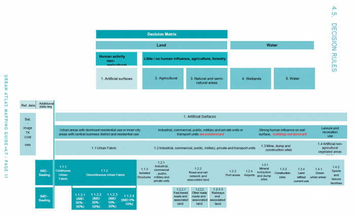
Before starting to map land cover classes using Sentinel-2 satellite images we need clear definitions and a classification scheme. An example for a hierarchical land use and land cover (LUC) classification scheme is the European Urban Atlas. The scheme defines 5 meta classes where the class 1. Artificial surfaces has many sub classes as shown in figure A.
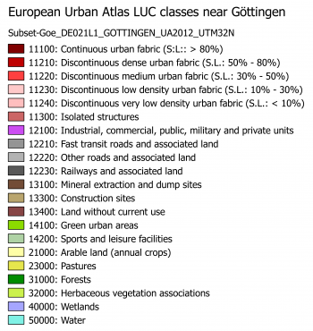
The specification of other meta classes is not as detailed. If we are more interested in forest and open area classes we need to adapt and modify this scheme. On the lowest level not all classes defined in the European Urban Atlas do also appear in the surroundings of Göttingen (figure B). In addition we need to consider the phenolgical development of vegetation at specific acquisiton dates and to specify more classes which can possibly be identified in multispectral feature space of the satellite image. An example of an adapted simplified scheme is shown in the table below.
| MC ID | MC info | C ID | C info | RGB code |
|---|---|---|---|---|
| 1 | Artificial surfaces | 11 | Built-up | 230-0-77 |
| 2 | Agricultural | 22 | Arable land | 255-255-168 |
| 2 | Agricultural | 23 | Bare soil | 253-191-168 |
| 2 | Agricultural | 24 | Pasture | 230-230-77 |
| 3 | Natural and semi-natural areas | 31 | Broad leaved tree cover | 128-255-0 |
| 3 | Natural and semi-natural areas | 32 | Coniferous tree cover | 0-166-0 |
| 5 | Water | 51 | Water | 128-242-230 |
| 6 | Miscellaneous | 61 | Cloud | 255-255-255 |
| 6 | Miscellaneous | 62 | Cloud shadow | 100-50-0 |
| 6 | Miscellaneous | 63 | Unclassified | 0-0-0 |

