Linear regression
Contents |
General observations
The direct observation of some tree variables, such as tree volume, but also tree height, is time consuming and therefore expensive. Thus, we may establish a statistical relationship between the target variable and variables that are easier to observe such as dbh. These relationships are formulated as mathematical functions which are used as prediction models: they allow us predicting the value of the target variable (dependent variable) once the value of the easy-to-measure variable (independent variable) is known. In forest inventory, two important models exist:
- height curves which predict the tree height from \(dbh:height=f(dbh)\) and
- volume functions which predict tree volume from \(dbh\) or from \(dbh\) and height or from other sets of independent variables:
- \(volume=f(dbh)\), or
- \(volume=f(\mbox{dbh, height})\), or
- \(volume=f(\mbox{dbh, upper diameter, height})\).
In order to build these models, one needs to define a mathematical function that shall be used, and one needs to select a set of sample trees at which all variables (the dependent variable and the independent variables) are observed. Then, the model has to be fitted to the sample data in a way that prediction errors are minimized. The resulting function with the best fit is then used as prediction model.
The mathematical principle of linear regression
The fundamental concept of regression is to establish a statistical relationship between dependent and independent variables such that predictions of the dependent variable can be done. What we look at here is the linear regression which uses mathematical models in which the coefficients are combined by linear operations. The variables need to be continuous and on a metric scale.
One should be clear that the predicted value is, of course, not the true value of the dependent variable of a particular tree, but it should be interpreted as the mean value of all trees with the same value for the independent variable. That means, the prediction read from a regression is rather an estimation than a measurement! We do illustrate the principle of regression for the simple linear regression, that is for the model
\(y=b_0+b_1x\,\),
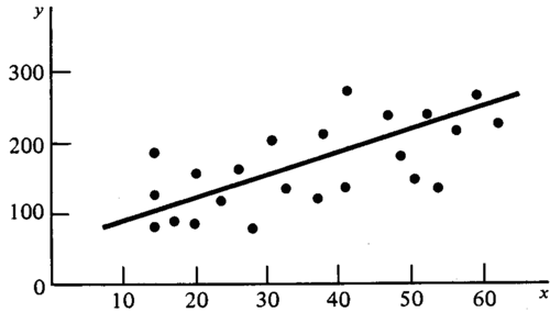
where \(y\) is the dependent variable and \(x\) the independent variable. The graphical representation of this model is a straight line (Figure 1).
With the statistical technique of regression analysis, the regression coefficients \(b_0\) and \(b_1\) are determined such that the regression curve (in this case the straight line) fits best to the given data. Of course, a criterion must be defined what the “best” curve and the optimal fit is. In general, the best curve will have some property like that the data points are as close as possible to the regression curve; in regression analysis this is defined as: the best fit is that of the regression curve for which the sum of the squared distances between data points and regression curve is a minimum. This technique is also called the “least squares method”.
