Geometric corrections
| Line 95: | Line 95: | ||
= Geometric Corrections = | = Geometric Corrections = | ||
| − | The geometric correction is done by describing the impacts of the distortions using sensor models in | + | The geometric correction is done by describing the impacts of the distortions using sensor models in four steps: |
| − | == Acquisition of ground control points (GCPs)== | + | == 1. Acquisition of ground control points (GCPs)== |
GCP's are either two (X,Y) or three (X,Y,Z) dimensional points for which both, the image coordinates (x,y,z) and the map coordinates (X,Y,Z) are known | GCP's are either two (X,Y) or three (X,Y,Z) dimensional points for which both, the image coordinates (x,y,z) and the map coordinates (X,Y,Z) are known | ||
| Line 111: | Line 111: | ||
| − | == Building a Sensor Model == | + | == 2. Building a Sensor Model == |
Sensor models formulate the relation between the image pixel coordinates (<math>c,r</math>) and the map coordinates (<math>X,Y</math>). For the models, it can be distinguished between ''image to ground''- forward models and ''ground to image''- inverse models. They can be expressed as: <math>X=f_x(c,r,h,\vec{\Theta})\\ | Sensor models formulate the relation between the image pixel coordinates (<math>c,r</math>) and the map coordinates (<math>X,Y</math>). For the models, it can be distinguished between ''image to ground''- forward models and ''ground to image''- inverse models. They can be expressed as: <math>X=f_x(c,r,h,\vec{\Theta})\\ | ||
| Line 139: | Line 139: | ||
Empirical approaches are used when no physical model or no a priori information for parametrization (e.g. about sensor, platform , Earth) is available. This empirical approaches are either based on polynomial models or rational functions. Empirical approaches are used when: no physical model is available, or when no a priori information for parameterization (e.g. about sensor, platform , Earth) is available. {Limitations and Drawbacks of sensor models} There are two critical elements in orthorectification based on sensor modeling. First, the validity of the sensor models hast to be questioned. But often these models are provided by the sensor operators and are thus generally trustworthy. Second, the accuracy of the available elevation models is critical to the modeling, as accurate models can only be based on high quality elevation information. | Empirical approaches are used when no physical model or no a priori information for parametrization (e.g. about sensor, platform , Earth) is available. This empirical approaches are either based on polynomial models or rational functions. Empirical approaches are used when: no physical model is available, or when no a priori information for parameterization (e.g. about sensor, platform , Earth) is available. {Limitations and Drawbacks of sensor models} There are two critical elements in orthorectification based on sensor modeling. First, the validity of the sensor models hast to be questioned. But often these models are provided by the sensor operators and are thus generally trustworthy. Second, the accuracy of the available elevation models is critical to the modeling, as accurate models can only be based on high quality elevation information. | ||
| − | == Coordinate Transformation == | + | == 3. Coordinate Transformation == |
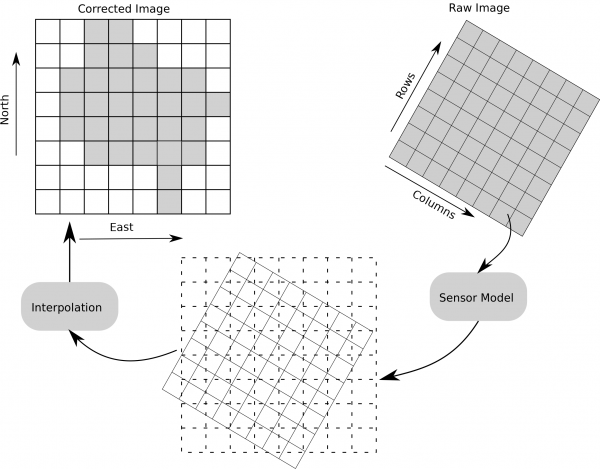
| − | [[File:Geometric_correction.png|600px|Figure 5: Coordinate Transformation]] | + | Once a suitable sensor model is defined it can be applied to the image raw data to calculate the corrected coordinates of the pixel locations as shown in Figure 5. |
| + | [[File:Geometric_correction.png|thumb|600px|Figure 5: Coordinate Transformation]] | ||
| − | == Resampling of Pixel Values == | + | == 4. Resampling of Pixel Values == |
| + | The coordinate transformations shifts and rotates the pixel locations. These new locations do not fit into a regular grid of the raster files. Therefore, the pixel values need to be resampled to assign each grid cell one raster values. There is a range of different resampling methods available, inluding: | ||
| + | * Nearest Neighbor | ||
| + | * Linear | ||
| + | * Cubic | ||
| + | * Cubic spline | ||
| + | [[File:Interpolation NN.png|600px|thumb|Figure 6: Nearest Neighbor Resampling]] | ||
[[Category:08 Image preprocessing]] | [[Category:08 Image preprocessing]] | ||
Latest revision as of 12:49, 30 September 2020
Author of this article: Paul Magdon
Contents |
[edit] Background
All remote sensing images of the Earth surface contain a significant amount of geometric distortions. The distortions are inherent in the acquisition geometry which is determined by the technical design of the observing unit (e.g. sensor and platform) and of the observed object (e.g. Earth surface), which can be summarized as sensor geometry. A spatial analysis of the images which includes the assessment of areas, distances, locations, angles and combinations with other spatial information by integrating the images into a geographic information system (GIS) is not ad hoc possible. Consequently, for a spatial image analysis a transformation of the sensor geometry into a meaningfull geometry with known geometric properties -- usually a form of a map projection -- is required. This transformation from sensor geometry to a map projection is referred to as geometric correction and is based on sensor models that reflect the nature and magnitude of distortions caused by the various sources such as Earth rotation, platform movement, and sensor errors.
[edit] Image Coordinate Systems
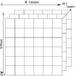
Digital images store the spectral information measured by a sensor into a format which can be read and analyzed by computers. The information is stored in a regular array of pixels which can be mathematically expressed as an \(N\times M\) matrix with \(x\) columns and \(y\) rows (see Fig.1). For each pixel one digital number (DN) is stored in the matrix. The image coordinate system is then defined by the origin \(x=0, y=0\) and the spacing of the pixels. The row indices start at the origin \((0,0)\) and increase downward, while the column indices increases to the right. Depending on the image format used, the origin can be located either in the center of the upper left pixel or at the upper left edge of that pixel. For multi-spectral images a third index \(b\) is introduced to represent the number of bands. Depending on the image format this starts either with \(0\) or \(1\).
[edit] Acquisition Geometry of Satellites
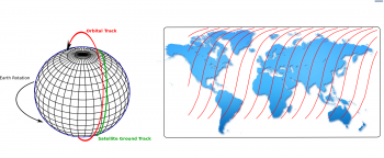
Different from geo-stationary orbits, where the satellites stay over the same location on Earth permanently (e.g. TV-broadcasting satellites), earth observation satellites should cover large areas of the Earth. Therefore, many of the satellite systems currently used for earth observation (e.g. Landsat, Sentinel, Planet) operate in a sun-synchronous orbit as shown in Fig. 2. In this orbit the satellites pass above or nearly above both pols of the Earth on each revolution. Due to the rotation of the earth the longitude at which the satellites cross over the equator shifts with each orbit, so that the full earth surface can be covered. Additionally, many of the optical earth observing satellites operate in sun-synchronous orbit, meaning that each successive orbit occurs at the same local time of day. Under this condition the illumination angle of the sun is kept constant.
Depending on the purpose, satellite systems are designed to operate in various acquisition modes. Two of the most common modes for optical sensors are along-track and cross-track acquisition.
- Cross-track scanners are based on one detector unit. The spatial coverage is achieved by using a rotating mirror which scans the surface perpendicular to the flight direction. Thus, the angular field of view is determined by the deflection of the mirror on the sensor altitude. Well known system using Cross-Track scanners are the Landsat family (MSS, TM, ETM+), MODIS and NOAA/AVHRR.
- Due to the rapid technical development of the detector units (CCD=Charge Couple Device) it became possible to combine many detectors in an array which resulted in a new generation of sensors called push-broom sensors. These sensors scan the surface parallel to the flight direction using a linear array of CCD’s aligned across-track. The image is build up by the movement of the platform. Using this technique, theoretically endless acquisition lines can be captured, thought data storage still limits the length of lines. Prominent along-track scanners are RapidEye, SPOT, ASTER, IKONOS,Quickbird and Geoeye.
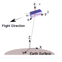
The acquisition geometry of the satellite systems can be described by the position of the sensor (x,y,z) the rotation parameters of the sensor (\(\phi,\omega,\kappa\)) and the surface coordinates given in a project map system (X,Y,Z) as depicted in Fig.3.
[edit] Sources of Image Distortion
Depending on the acquisition geometry and mode, different geometric distortions are inherent in the satellite raw data. Toutin (2003) categorized them as being either related to the observer or to the observed object. On the observer side the geometry is influences by the platform position (x,y,z) , the earth surface location and the sensor orientation (\(\phi,\omega,\kappa\)). A full nadir view is given when all rotation parameters are zero which minimize the images distortions. On the observed side, distortions are caused by the earth rotation and the relief displacement due to topography effects. Additionally, the Earth atmosphere can cause distortions by refraction of the electromagnetic waves. Table 1 summarizes the sources of image distortion.
| Category | Subcategory | Description | Error Type |
|---|---|---|---|
| Observer | Platform | Variations in platform movement | Systematic |
| Variations in platform attitude | Systematic | ||
| Sensor | Variations in sensor mechanics | Systematic | |
| View/look angles | Systematic | ||
| Panorama effect with field of view | Systematic | ||
| Onboard Measuring Instruments | Time-variations or drift | Random | |
| Clock-synchrony | Random | ||
| Observed | Earth | Curvature, rotation, topography | Systematic |
| Atmosphere | Refraction | Random | |
| Map | Geoid to ellipsoid, Ellipsoid to map | Systematic |
[edit] Geometric Corrections
The geometric correction is done by describing the impacts of the distortions using sensor models in four steps:
[edit] 1. Acquisition of ground control points (GCPs)
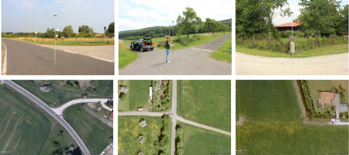
GCP's are either two (X,Y) or three (X,Y,Z) dimensional points for which both, the image coordinates (x,y,z) and the map coordinates (X,Y,Z) are known
- ideally as small as a single pixel
- high contrast to the surroundings
- constant location over time
Typical examples of GCP's are intersections of roads, distinctive water bodies, edges of land cover parcels and, corners of buildings.
[edit] 2. Building a Sensor Model
Sensor models formulate the relation between the image pixel coordinates (\(c,r\)) and the map coordinates (\(X,Y\)). For the models, it can be distinguished between image to ground- forward models and ground to image- inverse models. They can be expressed as\[X=f_x(c,r,h,\vec{\Theta})\\ Y=f_y(c,r,h,\vec{\Theta}) \]
In this equation \(\Theta\) represents a vector of parameters describing the image acquisition geometry and \(h\) gives the height typically derived from an elevation model.
Basically two types of sensor models can be differentiated: mechanistic and empirical models. The first are rigorous, complex models, where the parameters have a physical meaning (e.g distances, angles) which reconstruct the image geometry. This approach is used for example for SAR orthorectification based on the range-doppler model. The later approach, is an empirically approximate of the physical conditions. This is often done by expressing the parameters as polynomials or rations of polynomials the so-called ratio polynomial coefficients RPC which are sometimes also called replacement models. As these models are approximations, they are less accurate than the physical models, but they can be standardized and thus are easier to implement in remote sensing software.
[edit] Rigorous Sensor Models
The physical model should model all distortions of platform, sensor, Earth and cartographic projection based on measurable physical units. (degree, time, distance). This is typically achieved by using collinearity functions for optical data and the Rang-Doppler equation for RADAR images. Rigorous sensor models provide information about the sensors orbital movements. They describe the relationship between the image points and homologous ground points, with parameters which have understandable physical meanings using a collinear equation.
Adavantages:
- Useful when it is not possible to identify control points (e.g. to coarse resolution, little contrast,high cloud cover)
- Requires no human interaction
Disadavantages:
- Can only model systematic distortions
- Require complicate platform movement and position models
[edit] Non-Rigorous Models
Empirical approaches are used when no physical model or no a priori information for parametrization (e.g. about sensor, platform , Earth) is available. This empirical approaches are either based on polynomial models or rational functions. Empirical approaches are used when: no physical model is available, or when no a priori information for parameterization (e.g. about sensor, platform , Earth) is available. {Limitations and Drawbacks of sensor models} There are two critical elements in orthorectification based on sensor modeling. First, the validity of the sensor models hast to be questioned. But often these models are provided by the sensor operators and are thus generally trustworthy. Second, the accuracy of the available elevation models is critical to the modeling, as accurate models can only be based on high quality elevation information.
[edit] 3. Coordinate Transformation
Once a suitable sensor model is defined it can be applied to the image raw data to calculate the corrected coordinates of the pixel locations as shown in Figure 5.
[edit] 4. Resampling of Pixel Values
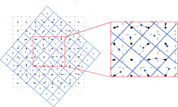
The coordinate transformations shifts and rotates the pixel locations. These new locations do not fit into a regular grid of the raster files. Therefore, the pixel values need to be resampled to assign each grid cell one raster values. There is a range of different resampling methods available, inluding:
- Nearest Neighbor
- Linear
- Cubic
- Cubic spline
