Change detection
(→Raster algebra: Difference) |
(→Raster algebra: Difference) |
||
| Line 50: | Line 50: | ||
[[File:Qgis_radio_ndwi.png|200px]] | [[File:Qgis_radio_ndwi.png|200px]] | ||
* Calculate also the NDWI for Landsat images '''SUB_LT5_2006-06-11_MUL.tif''' and '''SUB_LT5_2010-07-08_MUL.tif'''. | * Calculate also the NDWI for Landsat images '''SUB_LT5_2006-06-11_MUL.tif''' and '''SUB_LT5_2010-07-08_MUL.tif'''. | ||
| − | * Calculate the difference between the NDWI 2010 and NDWI | + | * Calculate the difference between the NDWI 2010 and NDWI 2006 using the Raster Calculator. |
* Click {{mitem|text=Raster --> Raster calculator}}. | * Click {{mitem|text=Raster --> Raster calculator}}. | ||
* A difference NDMI is calaculated by the expression as shown below. | * A difference NDMI is calaculated by the expression as shown below. | ||
| Line 56: | Line 56: | ||
[[File:Qgis_raster_calc_diff.png|600px]] | [[File:Qgis_raster_calc_diff.png|600px]] | ||
# Mark the difference NDMI image right click {{mitem|text=Properties --> Metadata}} [[Image:QGIS_2.0_metadata_info.png|100px]]. In the "properties" window scroll down and report mean STATISTICS_MEAN and standdard deviation STATISTICS_STDDEV. | # Mark the difference NDMI image right click {{mitem|text=Properties --> Metadata}} [[Image:QGIS_2.0_metadata_info.png|100px]]. In the "properties" window scroll down and report mean STATISTICS_MEAN and standdard deviation STATISTICS_STDDEV. | ||
| − | * Find threshold values for forest change areas: Calculate thresholds mean +- 2 | + | * Find threshold values for forest change areas: Calculate thresholds mean +- 2 * stddev. |
* {{mitem|text=Properties --> Histogram}} to plot the difference histogram. | * {{mitem|text=Properties --> Histogram}} to plot the difference histogram. | ||
| + | {{mitem|text=Properties --> Histogram}} | ||
=== Raster algebra: Ratio === | === Raster algebra: Ratio === | ||
Revision as of 22:02, 13 January 2018
Contents |
Prerequisites of spatio-temporal image analysis
Correct the pixel intensities as much as possible for uninteresting differences:
- Sensor calibration
- Exact spatial co-registration of images (especially pixel-by-pixel comparision)
- Cloud and cloud shadow masking
- Haze reduction
- Atmospheric correction
- Topographic illumination correction (mountains)
- Clear definitions and classification scheme
Visualization of multi-temporal images
- Add subsets of 3 Landsat TM multispectral scenes of 1992 (SUB_LT4_1992-07-30_MUL.tif), 2006 (SUB_LT5_2006-06-11_MUL.tif)and 2010 (SUB_LT5_2010-07-08_MUL.tif) into the QGIS TOC.
- Create color composites RGB=(B5 SWIR-1),(B4 NIR), (B3 Red) following Changing Raster Layer Style of a multiband file.
- Select Web --> OpenLayers plugin --> Google Maps --> Google Satellite. If the Plugin doesn't exist you'll first have to install the Openlayers plugin using Plugins --> Manage and install plugins. A new Layer Google Maps is loaded. The project CRS is automatically set to WGS84/Pseudo Mercator (EPSG:3857). Drag and drop the Layer to the bottom of the TOC.
Globe plugin
- The Globe plugin is already installed. It just needs to be activated.
Plugins --> Manage and Install Plugins --> Installed. Click the checkbox or doubleclick the name Globe to activate the plugin.
- Plugins --> Globe --> Launch Globe. The Globe windows opens side by side to the map canvas.
- In the Globe viewer click on Globe settings
 . Switch off the atmosphere rendering by unchecking the box Sky. OK.
- Adjust the size of the Globe viewer to the same size as the map canvas.
- In the map canvas zoom in to a region of interest. Adjust the local histogram stretch for all layers in the TOC clicking
 (Raster Tools).
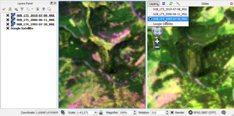
- In the Globe Viewer click on Layer Layer and check the layers that you would like to see oon top of the Globe Viewer. Attention uncheck the layer Google Satellite in the Globe Viewer: otherwise QGIS crashes!
- Click first on Reload layer
 and then Synchronize extent
  . The extents of the canvas and the Globe viewer are synchronized as shown below.
MapSwipe Tool plugin
This plugin is a map tool for swipe active layer, for example, you can see the difference with others layers below. The active layer, or group, will appear above all others.
- Select Plugins --> MapSwipe Tool or click
 . If the Plugin doesn't exist you'll first have to install it. Check Plugins --> Mange and Install plugins.. --> Settings Show also experimental plugins.
- Mark a layer below the top layer in the TOC and hold left click to blend to and compare two layers.
- Do not mark Google Satellite as active layer, otherwise QGIS crashes!
Temporal/Spectral Profile plugin
Change detection techniques
Bitemporal
Post-classification Comparison
This is an indirect change detection method: First two co-registered satellite images are independently classified to yield thematic maps. Then, discrete class labels of two thematic raster layers are compared to determine changes using cross-tabulation in which all transitions are presented. Use the Semi Automatic Classification plugin: Postprocessing --> Land cover change
Raster algebra: Difference
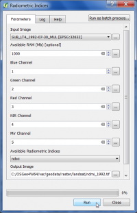
- In the search engine of the Processing Toolbox, type Radiometric and select Radiometric Indices under Feature Extraction of the Orfeo Toolbox.
- Select the Landsat TM SUB_LT4_1992-07-30_MUL.tif file as input layer.
- Assign the spectral bands to the right band number as shown below.
- Choose ndwi from the Available Radiometric Indices drop-down list to calculate the Normalized difference Water Index (NDWI). Synonyms are Normalized Difference Moisture Index (NDMI) and Normalized Difference Infrared Index (NDII).
- Enter name and path for an output file.
- Click on Run.
- Calculate also the NDWI for Landsat images SUB_LT5_2006-06-11_MUL.tif and SUB_LT5_2010-07-08_MUL.tif.
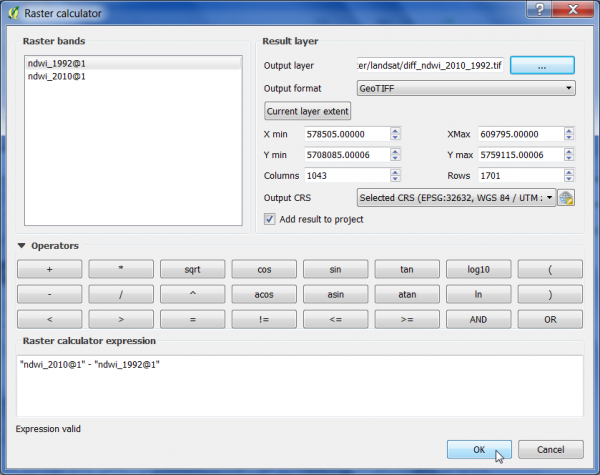
- Calculate the difference between the NDWI 2010 and NDWI 2006 using the Raster Calculator.
- Click Raster --> Raster calculator.
- A difference NDMI is calaculated by the expression as shown below.
- Define path and file name of the output layer. OK.
- Mark the difference NDMI image right click Properties --> Metadata
 . In the "properties" window scroll down and report mean STATISTICS_MEAN and standdard deviation STATISTICS_STDDEV.
- Find threshold values for forest change areas: Calculate thresholds mean +- 2 * stddev.
- Properties --> Histogram to plot the difference histogram.
Properties --> Histogram
Raster algebra: Ratio
- Open Toolbox --> OTB --> Feature Extraction --> Radiometric indices.
- Set tm_920526_mul.tif as Input Image.
- Set Red Channel to 4 and NIR Channel to 5.
- Set Available Radiometric Indices to ndvi.
- Save the Output Image as ndvi1992.
- Repeat this procedure for the raster file of 2005 and adapt the name of the Output Image to ndvi_2005.
- Calculate the ratio of both raster images with the Raster --> Raster Calculator.
- Choose ndvi_2005 from the Raster bands by double clicking on the raster name.
- Choose the division operator from the Operators by clicking on /.
- Choose ndvi_1992.tif from the Raster bands by double clicking on the raster name.
- Save the Output layer as ndvi_ratio and press OK.
Multi-temporal
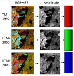
Multi-temporal color composite
- Add the raster layers of the years 1992 (tm_920526_mul.tif), 2000 (etm_000515_mul.tif) and 2005 (etm_050623_mul.tif) into a QGIS project. It should be available in the course data.
- Open Toolbox --> OTB --> Miscellaneous --> Band Math.
- Calculate the amplitude for each raster layer (1992, 2000, 2005) with the use of the bands 5-4-3.
- For the year 1992, set tm_920526_mul.tif as Input image list.
- Type sqrt(im1b4^2 + im1b5^2 + im1b3^2) as Expression.
- Save theOutput image as amplitude1992.
- Repeat this procedure for the raster files of 2000 and 2005 and adapt the name of each Output Raster File.
- Merge the three output raster files with Toolbox --> GDAL/OGR --> [GDAL] Miscellaneous --> Merge
- Load the three amplitude****.tif files as Input Layers, mark Layer Stack and save Merged output as amplitude_merge.
Principal component analysis
- Add the raster layers of the years 1992 (tm_920526_mul.tif), 2000 (etm_000515_mul.tif) and 2005 (etm_050623_mul.tif) into a QGIS project. It should be available in the course data.
- Install PCA plugin under Plugins --> Manage and Install Plugins....
- Open PCA plugin
 .
.
- Set tm_920526_mul.tif as Input Raster File.
- Set Number of output Principal Components to 1.
- Save the Output Raster File as pca1992_1.
- Repeat this procedure for the raster files of 2000 and 2005 and adapt the name of each Output Raster File.
- Merge the three output raster files with Toolbox --> GDAL/OGR --> [GDAL] Miscellaneous --> Merge.
- Load the three pca****_1.tif files as Input Layers, mark Layer Stack and save Merged output as pca_merge.


