Unsupervised classification (Tutorial)
From AWF-Wiki
(Difference between revisions)
| Line 78: | Line 78: | ||
##* Don't forget to click {{button|text=Classify}} for adding the classes. | ##* Don't forget to click {{button|text=Classify}} for adding the classes. | ||
## Click {{button|text=Load}} and confirm with {{button|text=Apply}} or {{button|text=OK}}. | ## Click {{button|text=Load}} and confirm with {{button|text=Apply}} or {{button|text=OK}}. | ||
| + | |||
| + | ==Figures== | ||
| + | {| class="wikitable" style="border:0pt" | ||
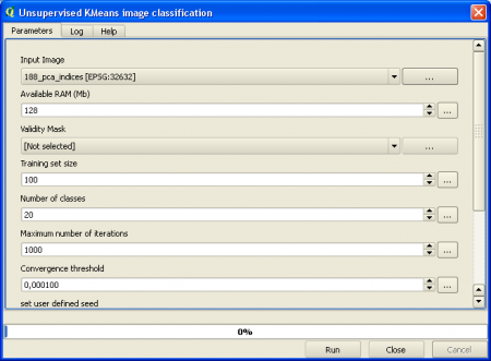
| + | |style="border:0pt"|[[Image:RemSens_Exercise07_01.png|thumb|450px|'''Figure A:''' Dialogue of the ''Unsupervised K-Means image classification'' plugin from the Orfeo toolbox in [[QGIS]].]] | ||
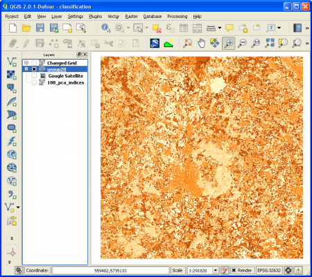
| + | |style="border:0pt"|[[Image:RemSens_Exercise07_02.png|thumb|450px|'''Figure B:''' Land cover map produced by the k-means clustering algorithm.]] | ||
| + | |- | ||
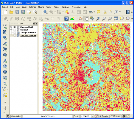
| + | |style="border:0pt"|[[Image:RemSens_Exercise07_03.png|thumb|450px|'''Figure C:''' Land cover map produced by the k-means clustering algorithm in discrete colors.]] | ||
| + | |} | ||
Revision as of 11:31, 17 February 2014
| sorry: |
This section is still under construction! This article was last modified on 02/17/2014. If you have comments please use the Discussion page or contribute to the article! |
- This article is part of the QGIS tutorial 2013/14.
In this article, you will learn how to classify a landscape raster via k-means clustering
| Code | Name | Cluster number | RGB color |
|---|---|---|---|
| 1 | Urban area | 10,9,15 | 230-000-077 |
| 2 | Cropland | 16,0,13,3,7,17,18 | 255-255-268 |
| 3 | Pastures/grassland | 12,8 | 230-230-077 |
| 4 | Broadleave forest | 6,2,5,4 | 128-255-000 |
| 5 | Coniferous forest | 11,19 | 000-166-000 |
| 6 | Water bodies | 14 | 128-242-230 |
| 7 | Cloud | 1 | 255-255-255 |
- Classifying an image
- Add the raster layer 188_pca_indices.tif into a QGIS project. It should be available in the course data.
- Open the k-means classification algorithm provided by the Orfeo toolbox. It can be found in the processing toolbar under Toolbox --> Orfeo Toolbox --> Learning --> Unsupervised KMeans image classification.
- Set the 188_pca_indices layer as Input image
- Set the Number of classes to 20 and the Number of iterations to 1000.
- The Convergence threshold should be set at 0.0001.
- Leave all other configurations as they are and click Run. The resulting image has 20 classes, labeled from 0 to 19.
- Image symbology
- Right-click the classified layer in the TOC and select Properties --> Style.
- Set the Render type to Singleband pseudocolor.
- Set the Mode to Equal interval with 20 classes and confirm with Classify.
- In the Load min/max section, select tbe Min/max radio button and click Load to update the range for classification.
- Confirm with Apply or click OK if you are content with your settings.
- Create a land use/cover classification scheme table as in table A
- As a reference, you may add a google layer to the project:
Plugins --> ObenLayers plugin --> Add Google Satellite layer - Set the coordinate reference system
- Open Project --> Project properties.
- Set WGS 84 Pseudo Mercarot (EPSG 3857) as coordinate system
- Check the Enable on the fly transformation box
- Right click 188_pca_indices in the TOC and select Set Project CRS from layer.
- Change the grid values
- Assign discrete colors to the land cover layer
- Right click the layer in the TOC or double click to open the layer Properties.
- Select the Style tab and set the following options:
- For Render type select Singleband pseudocolor
- For Color interpolation, select Discrete
- Set Mode to Equal interval and Classes to 7.
- Set Load min/max values to Min/max.
- Don't forget to click Classify for adding the classes.
- Click Load and confirm with Apply or OK.
Figures
 Figure A: Dialogue of the Unsupervised K-Means image classification plugin from the Orfeo toolbox in QGIS. |
|

