Exercise 09: Segmentation algorithms
From AWF-Wiki
(Difference between revisions)
| (12 intermediate revisions by 3 users not shown) | |||
| Line 1: | Line 1: | ||
| − | + | ==Preparatory steps== | |
| − | + | # Open image ''svm_classification.tif'' | |
| − | + | # Open the layer properties (right click in [[TOC]] or double click). In the {{button|text=Style}} tab, click {{button|text=Load style}} and browse for ''classification.qml''. | |
| − | + | # Open {{mitem|text=Plugins --> Openlayers plugin --> Add Google Satellite Layer}} (figure '''A'''). | |
| − | + | # With the image ''svm_classification.tif'' on top (with transparency more than 50%) we can compare the classification with the information of the Google image and look for errors in the classification (figure '''B'''). | |
| − | + | ||
| − | + | ||
# Improving the classification | # Improving the classification | ||
## Open {{mitem|text=Processing tools --> Orfeo Toolbox --> Classification Regularization}} | ## Open {{mitem|text=Processing tools --> Orfeo Toolbox --> Classification Regularization}} | ||
| − | ## Using the ''svm_classification.tif'' as input image run the classification regularization. Then you can compare the result to the image ''svm_classification.tif'' | + | ## Using the ''svm_classification.tif'' as input image run the classification regularization. See figure '''C''' for the parameter configuration. Then you can compare the result to the image ''svm_classification.tif'' (figure '''D'''). |
| − | + | # Installing Monteverdi | |
| − | # | + | #* Open {{mitem|text=Start --> OSGeo4W --> Setup}}. Select {{button|text=Advanced Install}} and {{button|text=Install from internet}} in the following window and confirm the default settings in the next four dialogues until reaching the {{button|text=Select package dialogue}}. Select Monteverdi from the software list (figure '''D'''). Confirm with {{button|text=Next}} |
| − | #* Open {{mitem|text=Start --> OSGeo4W --> Setup}}. Select {{button|text=Advanced Install}} and {{button|text=Install from internet}} in the following window and confirm the default settings in the next four dialogues until reaching the {{button|text=Select package dialogue}}. Confirm with {{button|text=Next}} | + | |
<!--(Please refer to Pool of figures 3 for the selected parameters information)--> | <!--(Please refer to Pool of figures 3 for the selected parameters information)--> | ||
| − | + | ||
| − | + | ==Segmentation in Monteverdi== | |
| − | + | # Open Monteverdi by double-clicking the icon on the Desktop | |
| − | + | # Select {{mitem|text=File --> Open dataset}} and browse for ''188_pcs_indices.tif'' | |
| − | + | # Open the panchromatic image saved in ''landsat8/DOY88/SUB_LC81950242013188LGN00_B8.tif'' via {{mitem|text=File --> Open dataset}}. | |
| − | + | # In order to equalize the spatial extent and resolution of the two maps, select {{mitem|text=Geometry --> Superimpose two images}} Select image ''188_pcs_indices.tif)'' for reprojection and ''SUB_LC81950242013188LGN00_B8.tif'' as reference image. Confirm with {{button|text=OK}}. | |
| − | + | # To generate an image with the characteristics of the multispectral image with the panchromatic resolution, select {{mitem|text=Filtering --> Pansharpening --> Simple RCA Pansharpening}} Select image to reproject (''188_pcs_indices.tif'') and the reference image for reprojection (''SUB_LC81950242013188LGN00_B8.tif''). Confirm with {{button|text=OK}}. | |
| − | + | # Save the processed image: Right-click the file of the output image (Pan SharpenedImageOutput) and select {{mitem|text=Export dataset --> pansharpened188.tif (32 bit)}}. Confirm with {{button|text=OK}}. | |
| − | + | # Load the generated image (''pansharpened188.tif'') into the [[QGIS]] project and compare it to the original multispectral image (''188_pcs_indices.tif''). | |
| − | + | # As segmentation is a procedure that requires high computational capacity, it is recommended o select a subset of the sharpened images: Select {{mitem|text=File --> Extract ROI from dataset}} and select the image ''pansharpened188.tif'' as input. Draw a box in the {{button|text=select ROI}} window and confirm with {{button|text=OK}} (figure '''F'''). | |
| − | + | # Applying the segmentation algorithm: | |
| − | + | # Open {{button|text=Filtering --> Mean shift clustering}} and select the ROI extracted from ''pansharpened188.tif''. Once you see the {{button|text=Mean shift module}} window you can change the parameters spectral value, spatial radius and opacity to find the pool of values that fit best to the characteristics of the image (e.g. figure '''G'''). | |
| − | + | # When the set of values that best fit to the image are found, the segmentation parameters can be applied to the whole image via {{button|text=Processing}}: Select {{mitem|text=Processing --> Orfeo Toolbox --> Segmentation --> Mean Shift segmentation (large scale, vector output)}}. Use ''pansharpened188.tif'' as input map with the parameters selected in {{button|text=Mean Shift module}} from Monteverdi software. | |
| − | + | ||
| − | + | ==Cloud detection in satellite images== | |
| − | + | # Load the raster image file ''188_pca_indices.tif'' from the ''supervised'' folder of the [[course data]]. | |
| − | + | # Load the raster image file ''SUB_LC81950242013188LGN00_B1.tif'' from ''geodata/raster/landsat/landsat8/DOY188'' folder into the project. (Coastal Aerosol Band) | |
| − | + | # Load the raster image file ''SUB_LC81950242013188LGN00_B11.tif'' from ''geodata/raster/landsat/landsat8/DOY188'' folder in QGis. (Thermal Infrared Band). Place the Band 11 image at the top in the [[TOC]]. | |
| − | + | # Generate a ratio channel with the raster calculator from {{mitem|text=Processing Toolbox --> SAGA --> Grid-Calculus --> Raster calculator}}. Select the raster images from Band 11 and 1. The formula must be a / b. Don't forget to enter the name for the image result. Start the calculation with {{button|text=Run}}. | |
| − | + | # Open the ratio image ''ratio_band11_band1.tif'' in Monteverdi via {{mitem|text=File --> Open dataset}}. | |
| − | + | # For filtering the image, select {{mitem|text=Filtering --> Threshold}} and select the ratio image generated in the previous step. Confirm with {{button|text=OK}}. | |
| − | + | # In the Threshold Module window select {{button|text=Binary Threshold}}; set outside value to {{typed|text=1}} and inside value to {{typed|text=0}}; Change the values of {{button|text=lower}} and {{button|text=upper}} threshold until the clouds are entirely covered (figure '''H'''). Save the threshold information. | |
| − | + | # Export the image: Select the output image with right clicking and selecting {{button|text=Export dataset}}. Save the output as ''cloud_mask.tif''. | |
| − | + | # Open the ''cloud_mask.tif'' image in QGis | |
| − | + | # Convert the image to shapefile: select {{mitem|text=Processing --> SAGA --> Shapes – Grid --> Vectorising Grid classes}}. Select the image. | |
| − | + | # To calculate the area of the polygons in the shapefile: Select {{mitem|text=Vector --> Geometry tools --> Export/ Add Geometry Columns}} | |
| + | # Open the attribute table of the shapefile and shift to editing mode. Press the icon of {{button|text=Select features using an expression}} and enter {{typed|text=area < 30000}}. Select and delete the selection. | ||
| + | # Place the image and ''188_pca_indices.tif'' on top of each other to see the final result of the clouds delineated (figure '''I'''). | ||
| + | |||
| + | ==Figures== | ||
| + | {| class="wikitable" style="border:0pt" | ||
| + | |style="border:0pt"|[[Image:RemSens_Exercise09_01.png|thumb|450px|'''Figure A''': Land cover map with underlying Google satellite layer.]] | ||
| + | |style="border:0pt"|[[Image:RemSens_Exercise09_02.png|thumb|450px|'''Figure B''': Zoom in on land cover map with underlying Google satellite layer. Note how forested areas are classified as water.]] | ||
| + | |style="border:0pt"|[[Image:RemSens_Exercise09_03.png|thumb|450px|'''Figure C''': ''Classification Regularization'' algorithm of the Orfeo Toolbox in [[QGIS]].]] | ||
| + | |- | ||
| + | |style="border:0pt"|[[Image:RemSens_Exercise09_04.png|thumb|450px|'''Figure D''': Land cover map before and after processing with the ''Classification Regularization'' plugin.]] | ||
| + | |style="border:0pt"|[[Image:RemSens_Exercise09_05.png|thumb|450px|'''Figure E''': OSGeo4W setup dialogue for installing software from the internet with row for ''Monteverdi'' highlighted.]] | ||
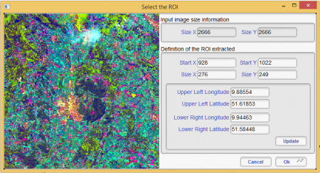
| + | |style="border:0pt"|[[Image:Monteverdi_Select_ROI.png|thumb|450px|'''Figure F''': The ''Select ROI'' module menu in Monteverdi.]] | ||
| + | |- | ||
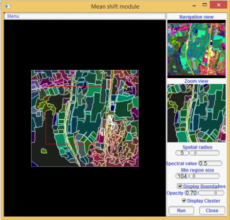
| + | |style="border:0pt"|[[Image:Monteverdi_Mean_shift.png|thumb|450px|'''Figure G''': The ''Mean shift'' module menu in Monteverdi.]] | ||
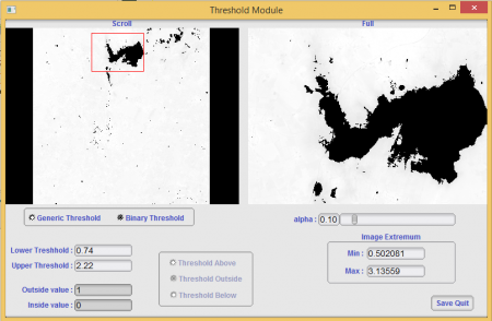
| + | |style="border:0pt"|[[Image:Monteverdi_Threshold.png|thumb|450px|'''Figure H''': The ''Threshold'' module menu in Monteverdi.]] | ||
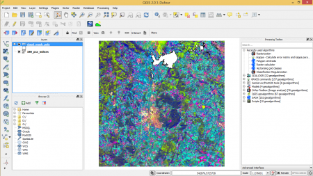
| + | |style="border:0pt"|[[Image:RemSens_Exercise09_10.png|thumb|450px|'''Figure I''': PCA Indices map and cloud vector layer.]] | ||
| + | |} | ||
Latest revision as of 09:57, 6 January 2020
Contents |
[edit] Preparatory steps
- Open image svm_classification.tif
- Open the layer properties (right click in TOC or double click). In the Style tab, click Load style and browse for classification.qml.
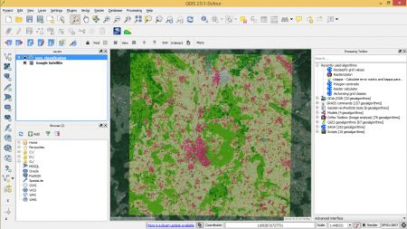
- Open Plugins --> Openlayers plugin --> Add Google Satellite Layer (figure A).
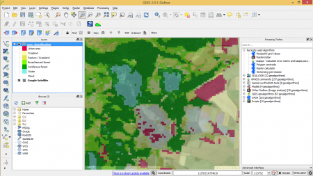
- With the image svm_classification.tif on top (with transparency more than 50%) we can compare the classification with the information of the Google image and look for errors in the classification (figure B).
- Improving the classification
- Open Processing tools --> Orfeo Toolbox --> Classification Regularization
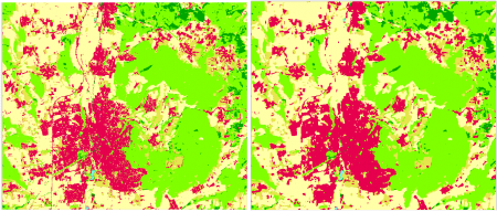
- Using the svm_classification.tif as input image run the classification regularization. See figure C for the parameter configuration. Then you can compare the result to the image svm_classification.tif (figure D).
- Installing Monteverdi
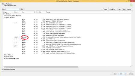
- Open Start --> OSGeo4W --> Setup. Select Advanced Install and Install from internet in the following window and confirm the default settings in the next four dialogues until reaching the Select package dialogue. Select Monteverdi from the software list (figure D). Confirm with Next
[edit] Segmentation in Monteverdi
- Open Monteverdi by double-clicking the icon on the Desktop
- Select File --> Open dataset and browse for 188_pcs_indices.tif
- Open the panchromatic image saved in landsat8/DOY88/SUB_LC81950242013188LGN00_B8.tif via File --> Open dataset.
- In order to equalize the spatial extent and resolution of the two maps, select Geometry --> Superimpose two images Select image 188_pcs_indices.tif) for reprojection and SUB_LC81950242013188LGN00_B8.tif as reference image. Confirm with OK.
- To generate an image with the characteristics of the multispectral image with the panchromatic resolution, select Filtering --> Pansharpening --> Simple RCA Pansharpening Select image to reproject (188_pcs_indices.tif) and the reference image for reprojection (SUB_LC81950242013188LGN00_B8.tif). Confirm with OK.
- Save the processed image: Right-click the file of the output image (Pan SharpenedImageOutput) and select Export dataset --> pansharpened188.tif (32 bit). Confirm with OK.
- Load the generated image (pansharpened188.tif) into the QGIS project and compare it to the original multispectral image (188_pcs_indices.tif).
- As segmentation is a procedure that requires high computational capacity, it is recommended o select a subset of the sharpened images: Select File --> Extract ROI from dataset and select the image pansharpened188.tif as input. Draw a box in the select ROI window and confirm with OK (figure F).
- Applying the segmentation algorithm:
- Open Filtering --> Mean shift clustering and select the ROI extracted from pansharpened188.tif. Once you see the Mean shift module window you can change the parameters spectral value, spatial radius and opacity to find the pool of values that fit best to the characteristics of the image (e.g. figure G).
- When the set of values that best fit to the image are found, the segmentation parameters can be applied to the whole image via Processing: Select Processing --> Orfeo Toolbox --> Segmentation --> Mean Shift segmentation (large scale, vector output). Use pansharpened188.tif as input map with the parameters selected in Mean Shift module from Monteverdi software.
[edit] Cloud detection in satellite images
- Load the raster image file 188_pca_indices.tif from the supervised folder of the course data.
- Load the raster image file SUB_LC81950242013188LGN00_B1.tif from geodata/raster/landsat/landsat8/DOY188 folder into the project. (Coastal Aerosol Band)
- Load the raster image file SUB_LC81950242013188LGN00_B11.tif from geodata/raster/landsat/landsat8/DOY188 folder in QGis. (Thermal Infrared Band). Place the Band 11 image at the top in the TOC.
- Generate a ratio channel with the raster calculator from Processing Toolbox --> SAGA --> Grid-Calculus --> Raster calculator. Select the raster images from Band 11 and 1. The formula must be a / b. Don't forget to enter the name for the image result. Start the calculation with Run.
- Open the ratio image ratio_band11_band1.tif in Monteverdi via File --> Open dataset.
- For filtering the image, select Filtering --> Threshold and select the ratio image generated in the previous step. Confirm with OK.
- In the Threshold Module window select Binary Threshold; set outside value to 1 and inside value to 0; Change the values of lower and upper threshold until the clouds are entirely covered (figure H). Save the threshold information.
- Export the image: Select the output image with right clicking and selecting Export dataset. Save the output as cloud_mask.tif.
- Open the cloud_mask.tif image in QGis
- Convert the image to shapefile: select Processing --> SAGA --> Shapes – Grid --> Vectorising Grid classes. Select the image.
- To calculate the area of the polygons in the shapefile: Select Vector --> Geometry tools --> Export/ Add Geometry Columns
- Open the attribute table of the shapefile and shift to editing mode. Press the icon of Select features using an expression and enter area < 30000. Select and delete the selection.
- Place the image and 188_pca_indices.tif on top of each other to see the final result of the clouds delineated (figure I).
[edit] Figures
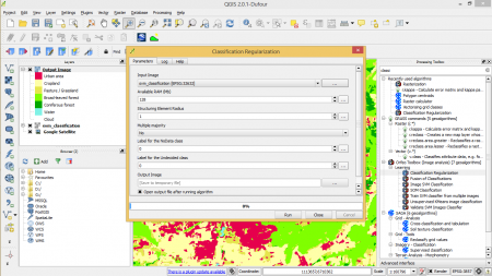 Figure C: Classification Regularization algorithm of the Orfeo Toolbox in QGIS. | ||
