Talk:Supervised classification (Tutorial)
From AWF-Wiki
(Difference between revisions)
(→GRASS implementation) |
(→Classification with Orfeo Toolbox (Outdated Qgis 2)) |
||
| (3 intermediate revisions by one user not shown) | |||
| Line 1: | Line 1: | ||
| + | == Image statistics(not mandatory, only if normalization of the variables is required) == | ||
| + | * Type into the search box of the Windows taskbar: {{typed|text=mapla.bat}}. Click on mapla.bat to open Monteverdi Application Launcher. | ||
| + | * In the search engine of mapla, type {{typed|text=ComputeImagesStatistics}} and double click '''ComputeImagesStatistics'''. | ||
| + | * Specify a multispectral image as Input Image: the Sentinel-2 image ''Subset_S2A_MSIL2A_20170619T_MUL_BOA.tif '' | ||
| + | * Specify directory and name for the XML Output image. Specify the extension '''.xml''' for this file. | ||
| + | * Click on {{button|text=Execute}}. | ||
| + | [[File:Qgis_ComputeImagesStatistics.png|500px]] | ||
| + | |||
| + | |||
| + | = Classification with Orfeo Toolbox (Outdated Qgis 2)= | ||
| + | == Image statistics == | ||
| + | # Add the Sentinel-2 imagery ''Subset_S2A_MSIL2A_20170619T_MUL_BOA.tif '' into a QGIS project. | ||
| + | # Calculate mean and standard error for each band of the Sentinel-2 imagery using the OTB Graphical User Interface. | ||
| + | * In the Search box on the Windows Start menu type {{typed|text=OSGeo4W Shell}}. You should be able to open the shell by clicking on it. | ||
| + | * Type into the shell: {{typed|text=otbgui_ComputeImagesStatistics}}. | ||
| + | Select a multiband input file and an output XML file as seen in the screenshot below. | ||
| + | [[File:Qgis_ComputeImagesStatistics.png|500px]] | ||
| + | |||
| + | == Train image classifier == | ||
| + | # Add the training areas as vector polygon file ''lab05_training_input.shp'' into QGIS. | ||
| + | # Open {{mitem|text=Orfeo Toolbox --> TrainImageClassifier (libsvm)}} to use the Support Vector Machine SVM algorithm (see figure '''B'''). | ||
| + | # Set ''Subset_S2A_MSIL2A_20170619T_MUL_BOA.tif'' as {{button|text=Input image list}}. | ||
| + | # Set ''lab05_training_input.shp'' as {{button|text=Input vector list}}. | ||
| + | # Set ''Subset_S2A_MSIL2A_20170619T_MUL_BOA.tif.xml'' as {{button|text=Input XML image statistics file}}. | ||
| + | # Set {{button|text=Name of discrimination field}} to ''C_ID'' (C_ID refers to the column that contains the LUC code). | ||
| + | # Save the {{button|text=Output confusion matrix}} as ''ConfusionMatrixSVM.csv''. | ||
| + | # Save the {{button|text=Output model}} as ''SVM.model''. | ||
| + | # Calculation of accuracies :<br/> Open ''ConfusionMatrixSVM.csv'' in LibreOffice or MS Excel and calculate overall, producer and consumer accuracies. | ||
| + | |||
| + | == Classification== | ||
| + | # Open {{mitem|text=Orfeo Toolbox --> Image Classification}} (see figure '''C'''). | ||
| + | # Set ''Subset_S2A_MSIL2A_20170619T_MUL_BOA.tif'' as {{button|text=Input image}}. | ||
| + | # Set ''SVM.model'' as {{button|text=Model file}}. | ||
| + | # Set ''Subset_S2A_MSIL2A_20170619T_MUL_BOA.xml'' as {{button|text=Statistical file}}. | ||
| + | # Save the {{button|text=Output image}} as ''su_svm.tif''. | ||
| + | # Evaluate classification results. | ||
| + | ## Add the classification result ''su_svm.tif'' to QGIS. | ||
| + | ## Right click ''su_svm.tif'' in the [[TOC]] and select {{mitem|text=Properties --> Style --> Style --> Load Style}}. | ||
| + | ## Load ''lab05_MinDist.qml''. | ||
| + | |||
| + | == Compute a confusion matrix with independent reference data == | ||
| + | # Open {{mitem|text=Orfeo Toolbox --> ComputeConfusionMatrix (Vector)}}. | ||
| + | # Set ''su_svm.tif'' as {{button|text=Input image}}. | ||
| + | # Set ''lab05_validation.shp'' as {{button|text=Input reference vector data}}. | ||
| + | # Set {{button|text=Field name}} to ''C_ID''. | ||
| + | |||
| + | |||
| + | |||
| + | |||
| + | |||
| + | |||
| + | |||
| + | |||
| + | |||
| + | |||
| + | |||
| + | |||
== GRASS implementation == | == GRASS implementation == | ||
When testing for GRASS in the Semi-Automatic Classification Plugin's | When testing for GRASS in the Semi-Automatic Classification Plugin's | ||
Latest revision as of 17:25, 8 December 2018
Contents |
[edit] Image statistics(not mandatory, only if normalization of the variables is required)
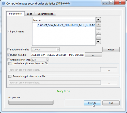
- Type into the search box of the Windows taskbar: mapla.bat. Click on mapla.bat to open Monteverdi Application Launcher.
- In the search engine of mapla, type ComputeImagesStatistics and double click ComputeImagesStatistics.
- Specify a multispectral image as Input Image: the Sentinel-2 image Subset_S2A_MSIL2A_20170619T_MUL_BOA.tif
- Specify directory and name for the XML Output image. Specify the extension .xml for this file.
- Click on Execute.
[edit] Classification with Orfeo Toolbox (Outdated Qgis 2)
[edit] Image statistics
- Add the Sentinel-2 imagery Subset_S2A_MSIL2A_20170619T_MUL_BOA.tif into a QGIS project.
- Calculate mean and standard error for each band of the Sentinel-2 imagery using the OTB Graphical User Interface.
- In the Search box on the Windows Start menu type OSGeo4W Shell. You should be able to open the shell by clicking on it.
- Type into the shell: otbgui_ComputeImagesStatistics.
Select a multiband input file and an output XML file as seen in the screenshot below.
[edit] Train image classifier
- Add the training areas as vector polygon file lab05_training_input.shp into QGIS.
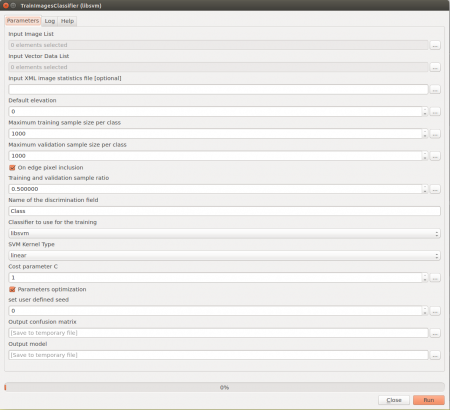
- Open Orfeo Toolbox --> TrainImageClassifier (libsvm) to use the Support Vector Machine SVM algorithm (see figure B).
- Set Subset_S2A_MSIL2A_20170619T_MUL_BOA.tif as Input image list.
- Set lab05_training_input.shp as Input vector list.
- Set Subset_S2A_MSIL2A_20170619T_MUL_BOA.tif.xml as Input XML image statistics file.
- Set Name of discrimination field to C_ID (C_ID refers to the column that contains the LUC code).
- Save the Output confusion matrix as ConfusionMatrixSVM.csv.
- Save the Output model as SVM.model.
- Calculation of accuracies :
Open ConfusionMatrixSVM.csv in LibreOffice or MS Excel and calculate overall, producer and consumer accuracies.
[edit] Classification
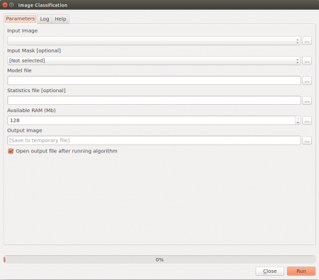
- Open Orfeo Toolbox --> Image Classification (see figure C).
- Set Subset_S2A_MSIL2A_20170619T_MUL_BOA.tif as Input image.
- Set SVM.model as Model file.
- Set Subset_S2A_MSIL2A_20170619T_MUL_BOA.xml as Statistical file.
- Save the Output image as su_svm.tif.
- Evaluate classification results.
- Add the classification result su_svm.tif to QGIS.
- Right click su_svm.tif in the TOC and select Properties --> Style --> Style --> Load Style.
- Load lab05_MinDist.qml.
[edit] Compute a confusion matrix with independent reference data
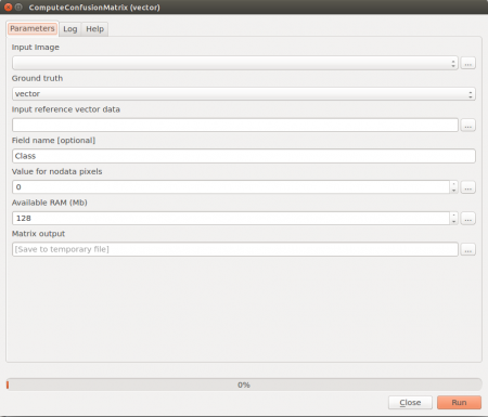
- Open Orfeo Toolbox --> ComputeConfusionMatrix (Vector).
- Set su_svm.tif as Input image.
- Set lab05_validation.shp as Input reference vector data.
- Set Field name to C_ID.
[edit] GRASS implementation
When testing for GRASS in the Semi-Automatic Classification Plugin's Settings tab, I needed to have grass set up first (i.e. created a grassdata folder with a location and mapset); this makes sense, but I don't know if we provide a tutorial for this yet? - Levent (talk) 17:22, 24 February 2014 (CET)
This Module does not work in QGIS 2.18-ltr:
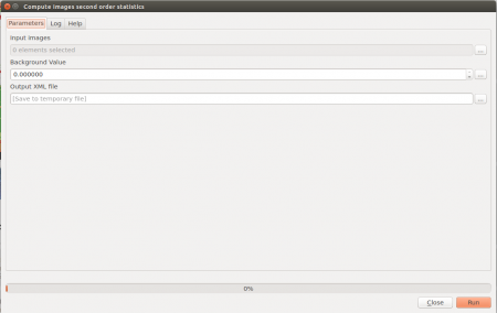
- Open Orfeo Toolbox --> Compute images second order statistics (see figure A).
- Set Subset_S2A_MSIL2A_20170619T_B12_BOA.tif as Input images.
- Save the Output XML file as Subset_S2A_MSIL2A_20170619T_B12_BOA.tif.xml.
Outdated figures:
