Region Growing Segmentation

Region Growing Segmentation with Saga's Seeded Region Growing Tool

The following tutorial by Sebastian Kasanmascheff explains how to delineate tree crowns, using SAGA's Seeded Region Growing Tool. The product, a polygon shapefile, can then be used in an object-based classification, f.ex. in order to classify different tree species.

Material you need to complete the tutorial

Data

A multispectral image of the forest canopy

A canopy height model CHM

Software

QGIS 2.18.11

SAGA 2.3.2

Split multiband image into several raster images

SAGA's Region Growing Algorithm works only with single band images. Therefor, we have to split our multiband image into its individual bands following these instructions.

Seed points

The first step here is to extract the position of the tree tops, which are going to be the starting point for the region growing algorithm. You find a description of how to derive the seed points from a CHM here . Now have a look at how the seeds align with your multiband image

In this picture you see, that the points align well with the tree tops. However, there are many points that represent small trees (in the lower left corner) which you might not be so interested in. In order to correct that, we are going to filter the points by their height in the seed shapefile and save the shapefile with the selected seeds only, as a new shapefile. If the seed points do not fit the image well, it might be due to the fact that you are using an orthophoto and not a true-orthophoto. If you are working only with a smaller dataset you can help it by using the Georeferencer in the Raster menu by rubbersheeting your orthophoto to make it fit. You'll find the instructions for doing so here.

This looks much better:

Seed point rasterization

In order to use the seed points in the region growing algorithm in SAGA, we have to convert the vector file to a raster file using the Rasterize module from the GDAL Conversions in QGIS. It is critical that we create a raster file that only contains the seed points and no-data. So every pixel outside the seed points has to be no-data. It is also critical that our rasterized vector image has the exact same CRS (Coordinate reference system), extent and pixel size as the single band images.

• In the Processing Toolbox, type 'rasterize' and select the Rasterize tool ind the SAGA geoalgorithms submenu
• Select the seed point shapefile as input
• Select ID as Attribute and the other parameters according to the screenshot below
• Select the extent of one of the band splits as extent by clicking select canvas/ layers extent in the Output extent line
• Copy the exact cellsize from either the metadata of one of your split images and set output raster size to Output resolution in map units per pixel
• Save to a local file

The result should look like this:

Now verify that the newly created seed point raster aligns 100% with one of the band split rasters by checking the metadata or the Save raster layer as.. mask and by zooming into the seed pixels. Also check with the Info button, if any pixel which is not a seed point, is no-data.

Your raster should align like this:

Superimpose Vector

It happens regularly that, although following the previous steps meticulously, that the extent and pixel size of the rasterized vector file does not match the splitted band images 100 %. In this case we have to use the OTB Superimpose Vector tool that you can find in the Processing Toolbox.

• Open the Superimpose Vector tool in the Processing Toolbox.
• Select one of the split band images as Reference input
• Select the rasterized seed point shapefile as The image to reproject
• Fill in the other parameters as shown here:

Next, go to the Properties of the newly created layer in the Layers Panel

• Check the extent of the layer in the Metadata tab.
• Go to Styles, load max/min values and set the Color Gradient to White to black

The result should look very much the same as the first rasterized vector, but the extent and pixel size are now 100 % the same as in

the split band images.

Region Growing in SAGA

Now we finally made it to the fun part of the whole exercise, which is creating the segments around the tops of the trees i.e. the seed points. Therefor we open SAGA GIS.

• When prompted, select an empty Startup Project

• Click the button

• Change to All files

• Open all split band images and the superimposed seed raster one after another
• The layer panel on the left should now look like this:

• In the line below Grids you see the extent of your raster files. If you happen to see two different of those lines, your raster images do not match 100 %. You can fix that again with the Superimpose sensor Tool in the OTB library in QGIS

Seeded Region Growing Algorithm

• Go to the Geoprocessing menu and select Find and Run tool

• Write ' region growing' and select

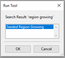
• Select the one grid on offer
• Select your seed point raster as Seeds

• Select your splitted band images as Features
• Select create in Segments, Similarity and Tables<<Seeds
• Select Normalize
• Select 4 (von Neumann
• Select feature space and position
• Insert the values shown in the picture and click Okay twice. We will talk about the input values later on...

After a short while, SAGA will have finished the calculation and you'll notice two new layers in the layer panel. Double-click on Segments and you hopefully see the first fruit of all the effort that you put into this exercise:

Vectorising the raster data

In the next step we are going to create polygons in a shapefile which we can then open in QGIS...

• In the Find and Run tool search, enter 'vectorising grid' and select

• Fill in the mask as follows and double-click Okay :

• Right click on the newly created Segments file under Shapes in the Layer panel
• Select Save as and save the file as ESRI shapefile

Opening the polygon file in QGIS

Now you can open the shapefile in QGIS and adjust the look of the segments in the Styles tab in the properties of the layer:

The math part

As you see in the last image, the segments fit the crowns quite well, but there is room for improvement. You can start to fine-tune the segmentation by changing the different parameters in the segmentation tool: Variance in Feature Space, Variance in Position Space, (Similarity Treshold), Method and Neighbourhood. You can also try to include or exclude certain data.

You can do that by trial and error, however, it helps to understand the math that lies behind these algorithms.

What the algorithm in the Seeded Region Growing module does, is that it starts with the seed point, goes to the adjacent pixels and joins them together if they are similar enough. 'Enough' in this case is determined by the similarity-condition which is expressed in the following formula:

The meaning of the parameters are easy to understand: 'f' is a value (f.ex. a spectral value or a height value) 'r' is a location. The indices designate which value it is, the one from the seed point or from the pixel that is being investigated (should it be joined to the segment of the seed or not). 't' indicates vector transposition and σ₁ and σ₂ are variances in colour and position space. The latter normalize the value differences between seed point and pixel. α is the similarity criterion. It not need to be normalized and is set arbitrarily at 0.15.

σ₁ and σ₂ control how far away the values (feature space / position space) are allowed to be between each other. For a maximum distance of 40 % of the peak intensity and three color bands, the formula for σ₁ is:

σ₂ determines the maximum spatial distance δ which is set to the radius of the largest crown (for spherical crowns):

(BECHTEL 2008)

The algorithm in the Seeded Region Growing module is based on the work of ERIKSON (2003, 2004, ERIKSON & OLOFSSON 2005)

References

- ↑ Bechtel, B. (2008)."Segmentation for Object Extraction of Trees using MATLAB and SAGA." SAGA–Seconds Out, Hamburger Beiträge Zur Physischen Geographie Und Landschaftsökologie. Univ. Hamburg, Inst. für Geographie (2008): 1-12..
- ↑ Erikson, M. (2003). Segmentation of individual tree crowns in colour aerial photographs using region growing supported by fuzzy rules. Canadian Journal of Forest Research, 33(8), 1557-1563.
- ↑ Erikson, M. (2004). Segmentation and classification of individual tree crowns (Vol. 320).
- ↑ Erikson, M., & Olofsson, K. 2005). Comparison of three individual tree crown detection methods. Machine Vision and Applications, 16(4), 258-265.